


Next: Periodic Driving Forces
Up: One-Dimensional Motion
Previous: Quality Factor
Resonance
We have seen that when a one-dimensional dynamical system is slightly perturbed
from a stable equilibrium point (and then left alone), it eventually returns to this point at
a rate controlled by the amount of damping in the system. Let us now
suppose that the same system is subject to continuous oscillatory constant amplitude
external forcing at some fixed frequency,  . In this
case, we would expect the system to eventually settle down to some steady oscillatory pattern of motion
with the same frequency as the external forcing. Let us investigate the properties of this type of driven oscillation.
. In this
case, we would expect the system to eventually settle down to some steady oscillatory pattern of motion
with the same frequency as the external forcing. Let us investigate the properties of this type of driven oscillation.
Suppose that our system is subject to an external force of the form
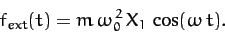 |
(104) |
Here,  is the amplitude of the oscillation at which the external force matches the restoring
force, (76). Incorporating the above force into our perturbed
equation of motion, (83), we obtain
is the amplitude of the oscillation at which the external force matches the restoring
force, (76). Incorporating the above force into our perturbed
equation of motion, (83), we obtain
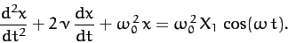 |
(105) |
Let us search for a solution of the form (84), and
represent the right-hand side of the above equation as
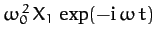 . It is again understood
that the physical solutions are the real parts of these expressions.
Note that is now a real parameter. We obtain
. It is again understood
that the physical solutions are the real parts of these expressions.
Note that is now a real parameter. We obtain
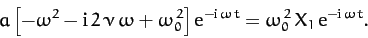 |
(106) |
Hence,
 |
(107) |
In general,  is a complex quantity. Thus, we can write
 |
(108) |
where  and
and  are both real. It follows from
Equations (84), (107), and (108) that the physical solution takes the
form
are both real. It follows from
Equations (84), (107), and (108) that the physical solution takes the
form
 |
(109) |
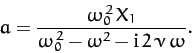
where
![\begin{displaymath}
x_1 = \frac{\omega_0^{\,2}\,X_1}{\left[(\omega_0^{\,2}-\omega^2)^2
+ 4\,\nu^2\,\omega^2\right]^{1/2}},
\end{displaymath}](img373.png) |
(110) |
and
 |
(111) |
We conclude that, in response to the applied sinusoidal force, (104), the system
executes a sinusoidal pattern of motion at the same frequency, with fixed amplitude , and phase-lag (with respect to
the external force).
Figure 6:
Resonance.
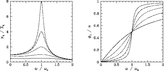 |
Let us investigate the variation of and with the forcing frequency,
. This is most easily done graphically. Figure 6 shows and as functions of for
various values of  . Here,
 ,
,  ,
,  ,
,  , and
, and  correspond to the solid, dotted, short-dashed, long-dashed,
and dot-dashed curves, respectively. It can be seen that as the amount of
damping in the system is decreased, the amplitude of the response becomes
progressively more peaked at the natural frequency of oscillation of the system,
correspond to the solid, dotted, short-dashed, long-dashed,
and dot-dashed curves, respectively. It can be seen that as the amount of
damping in the system is decreased, the amplitude of the response becomes
progressively more peaked at the natural frequency of oscillation of the system,  . This effect is known as resonance, and
is termed the resonant frequency. Thus,
a weakly damped system (i.e.,
. This effect is known as resonance, and
is termed the resonant frequency. Thus,
a weakly damped system (i.e.,
 ) can be driven to large amplitude by the application of a relatively
small external force which oscillates at a frequency close to the resonant frequency. Note that the response of the system is in phase (i.e.,
) can be driven to large amplitude by the application of a relatively
small external force which oscillates at a frequency close to the resonant frequency. Note that the response of the system is in phase (i.e.,
 )
with the external driving force for driving frequencies well below the resonant
frequency, is in phase quadrature
(i.e.,
)
with the external driving force for driving frequencies well below the resonant
frequency, is in phase quadrature
(i.e.,  )
at the resonant frequency, and is in anti-phase (i.e.,
)
at the resonant frequency, and is in anti-phase (i.e.,
 )
for frequencies well above the resonant frequency.
)
for frequencies well above the resonant frequency.
According to Equation (110),
 |
(112) |
In other words, the ratio of the driven amplitude at the resonant frequency
to that at a typical non-resonant frequency (for the same drive amplitude)
is of order the quality factor. Equation (110) also implies that,
for a weakly damped oscillator (
),
![\begin{displaymath}
\frac{x_1(\omega)}{x_1(\omega=\omega_0)}\simeq \frac{\nu}{[(\omega-\omega_0)^2 + \nu^2]^{1/2}},
\end{displaymath}](img385.png) |
(113) |
provided
 .
Hence, the width of the resonance
peak (in frequency) is
.
Hence, the width of the resonance
peak (in frequency) is
 , where the edges of peak are defined as the points at which the driven amplitude
is reduced to
, where the edges of peak are defined as the points at which the driven amplitude
is reduced to  of its maximum value. It follows that the
fractional width is
of its maximum value. It follows that the
fractional width is
 |
(114) |
We conclude that the
height and width of the resonance peak of a weakly damped ( ) oscillator scale as
  and
and
 , respectively. Thus, the area under the resonance curve stays
approximately constant as varies.
, respectively. Thus, the area under the resonance curve stays
approximately constant as varies.
Next: Periodic Driving Forces
Up: One-Dimensional Motion
Previous: Quality Factor
Richard Fitzpatrick
2011-03-31