 |
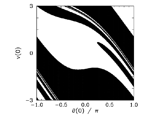
Figure 69 shows the basins of attraction, in ![]() -
-![]() space,
of the asymmetric mirror image attractors
pictured in Figures 66 and 67. The basin of attraction
of the left-favoring attractor shown in Figure 66 is coloured black, whereas
the basin of attraction
of the right-favoring attractor shown in Figure 67 is coloured white. It can
be seen that the two basins form a complicated interlocking pattern. Since we can
identify the angles
space,
of the asymmetric mirror image attractors
pictured in Figures 66 and 67. The basin of attraction
of the left-favoring attractor shown in Figure 66 is coloured black, whereas
the basin of attraction
of the right-favoring attractor shown in Figure 67 is coloured white. It can
be seen that the two basins form a complicated interlocking pattern. Since we can
identify the angles ![]() and
and ![]() , the right-hand edge of the pattern connects
smoothly with its left-hand edge. In fact, we can think of the pattern as existing
on the surface of a cylinder.
, the right-hand edge of the pattern connects
smoothly with its left-hand edge. In fact, we can think of the pattern as existing
on the surface of a cylinder.
 |
Suppose that we take a diagonal from the bottom left-hand corner of Figure 69 to its top right-hand corner. This diagonal is intersected by a number of black bands of varying thickness. Observe that the two narrowest bands (i.e., the fourth band from the bottom left-hand corner and the second band from the upper right-hand corner) both exhibit structure which is not very well resolved in the present picture.
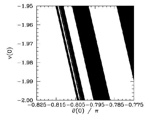 |
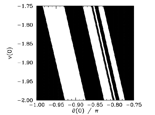
Figure 70 is a blow-up of a region close to the lower left-hand corner of Figure 69. It can be seen that the unresolved band in the latter figure (i.e., the second and third bands from the right-hand side in the former figure) actually consists of a closely spaced pair of bands. Note, however, that the narrower of these two bands exhibits structure which is not very well resolved in the present picture.
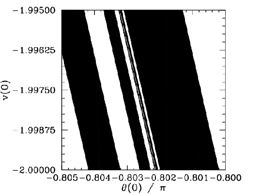 |
Figure 71 is a blow-up of a region of Figure 70. It can be seen that the unresolved band in the latter figure (i.e., the first and second bands from the left-hand side in the former figure) actually consists of a closely spaced pair of bands. Note, however, that the broader of these two bands exhibits structure which is not very well resolved in the present picture.
Figure 72 is a blow-up of a region of Figure 71. It can be seen that the unresolved band in the latter figure (i.e., the first, second, and third bands from the right-hand side in the former figure) actually consists of a closely spaced triplet of bands. Note, however, that the narrowest of these bands exhibits structure which is not very well resolved in the present picture.
It should be clear, by this stage, that no matter how closely we look at Figure 69 we are
going to find structure which we cannot resolve. In other words, the separatrix between the two
basins of attraction shown in this figure is a curve which exhibits structure at all
scales. Mathematicians have a special term for such a curve--they call it a
fractal.![[*]](footnote.png)
Many people think of fractals as mathematical toys whose principal use is the generation of pretty pictures. However, it turns out that there is a close connection between fractals and the dynamics of non-linear systems--particularly systems which exhibit chaotic dynamics. We have just seen an example in which the boundary between the basins of attraction of two co-existing attractors in phase-space is a fractal curve. This turns out to be a fairly general result: i.e., when multiple attractors exist in phase-space the separatrix between their various basins of attraction is invariably fractal. What is this telling us about the nature of non-linear dynamics? Well, returning to Figure 69, we can see that in the region of phase-space in which the fractal behaviour of the separatrix manifests itself most strongly (i.e., the region where the light and dark bands fragment) the system exhibits abnormal sensitivity to initial conditions. In other words, we only have to change the initial conditions slightly (i.e., so as to move from a dark to a light band, or vice versa) in order to significantly alter the time-asymptotic motion of the pendulum (i.e., to cause the system to converge to a left-favouring instead of a right-favouring attractor, or vice versa). Fractals and extreme sensitivity to initial conditions are themes which will reoccur in our investigation of non-linear dynamics.