Next: Flat Lifting Wings
Up: Two-Dimensional Compressible Inviscid Flow
Previous: Linearized Subsonic Flow
The aim of this section is to re-examine the problem of supersonic flow past a thin,
two-dimensional airfoil using the small-perturbation theory developed in Section 15.12.
As before, the unperturbed flow is of uniform speed  , directed parallel to the
  -axis, and the associated Mach number is
 .
The perturbed flow, due to the presence of the airfoil, is governed by Equation (15.127), which can be written in the hyperbolic
form (see Section 15.14)
.
The perturbed flow, due to the presence of the airfoil, is governed by Equation (15.127), which can be written in the hyperbolic
form (see Section 15.14)
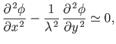 |
(15.183) |
where
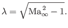 |
(15.184) |
As we saw in Section 15.14, the general solution of Equation (15.183) is
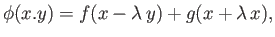 |
(15.185) |
where  and
and  are arbitrary functions. Because disturbances only propagate along downstream-running
Mach lines (i.e., Mach lines that originate at the airfoil), we only need the function
for the upper surface, and
the function
for the lower surface. Thus,
are arbitrary functions. Because disturbances only propagate along downstream-running
Mach lines (i.e., Mach lines that originate at the airfoil), we only need the function
for the upper surface, and
the function
for the lower surface. Thus,
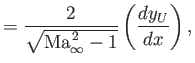
On the upper surface, the boundary condition (15.129) yields
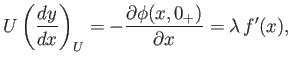 |
(15.188) |
which implies that
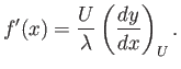 |
(15.189) |
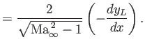
Similarly,
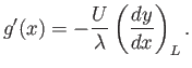 |
(15.190) |
According to Equation (15.128), the pressure coefficient on the surface of the airfoil is given by
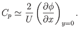 |
(15.191) |
Hence, we
obtain
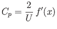 |
(15.192) |
on the upper surface, and
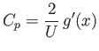 |
(15.193) |
on the lower surface. Thus,
This is the same result as that obtained in Section 15.9, where the pressure on thin airfoils was obtained by an
approximation to the shock-expansion method. In fact, for the purposes of calculating the velocity and pressure perturbations
on the surface of the airfoil, the linearized theory discussed in this section is equivalent to the weak wave approximations of Section 15.9.
Next: Flat Lifting Wings
Up: Two-Dimensional Compressible Inviscid Flow
Previous: Linearized Subsonic Flow
Richard Fitzpatrick
2016-03-31