Next: Exercises
Up: Two-Dimensional Potential Flow
Previous: Complex Line Integrals
Blasius Theorem
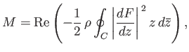
Consider some flow pattern in the complex  -plane that is specified by the complex velocity potential
  .
Let
.
Let  be some closed curve in the complex
-plane.
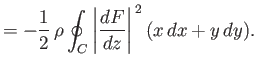
The fluid pressure on this curve is determined from Equation (6.41), which yields
be some closed curve in the complex
-plane.
The fluid pressure on this curve is determined from Equation (6.41), which yields
 |
(6.173) |
Let us evaluate the resultant force (per unit length), and the resultant moment (per unit length), acting on the fluid within the curve
as a consequence of this pressure distribution.
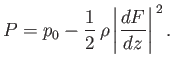
Figure 6.19:
Force acting across a short section of a curve.
 |
Consider a small element of the curve
, lying between  ,
,  and
and  ,
,  , which is sufficiently
short that it can be approximated as a straight-line. Let
, which is sufficiently
short that it can be approximated as a straight-line. Let  be the local fluid pressure on the outer (i.e., exterior to the curve) side of the element. As illustrated
in Figure 6.19, the pressure force (per unit length) acting inward (i.e., toward the inside of the curve) across the element has a component
be the local fluid pressure on the outer (i.e., exterior to the curve) side of the element. As illustrated
in Figure 6.19, the pressure force (per unit length) acting inward (i.e., toward the inside of the curve) across the element has a component  in the minus
-direction, and a component
in the minus
-direction, and a component  in the plus
-direction. Thus, if
in the plus
-direction. Thus, if  and
and  are the components of the
resultant force (per unit length) in the
- and
-directions, respectively, then
are the components of the
resultant force (per unit length) in the
- and
-directions, respectively, then
The pressure force (per unit length) acting across the element also contributes to a moment (per unit length),  , acting
about the
-axis, where
, acting
about the
-axis, where
 |
(6.176) |
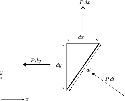
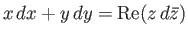
Thus, the
- and
-components of the resultant force (per unit length) acting on the of the fluid within the curve, as
well as the resultant moment (per unit length) about the
-axis, are given by
respectively,
where the integrals are taken (counter-clockwise) around the curve
. Finally, given that the pressure distribution on the curve takes the
form (6.173), and that a constant pressure obviously yields zero force and zero moment,
we find that
Now,
 , and
, and
 , where
  indicates a complex conjugate.
Hence,
indicates a complex conjugate.
Hence,
 , and
, and
 . It follows that
 |
(6.183) |
However,
 |
(6.184) |
where
 and
and
 . Suppose that the curve
corresponds to
a streamline of the flow, in which case
. Suppose that the curve
corresponds to
a streamline of the flow, in which case
 on
. Thus,
on
. Thus,  on
, and so
on
, and so
 .
Hence, on
,
.
Hence, on
,
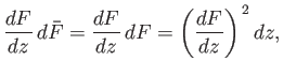 |
(6.185) |
which implies that
 |
(6.186) |
This result is known as the Blasius theorem, after Paul Blasius (1883-1970).
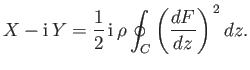
Now,
 . Hence,
 |
(6.187) |
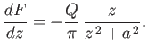
or, making use of an analogous argument to that employed previously,
![$\displaystyle M = {\rm Re}\left[-\frac{1}{2}\,\rho \oint_C \left(\frac{dF}{dz}\right)^{\,2} z\,dz\right],$](img2412.png) |
(6.188) |
In fact, Equations (6.186) and (6.188) hold even when  is not constant on the curve
, as long as
can be continuously deformed into a constant-
curve without leaving the fluid or crossing over a singularity of
is not constant on the curve
, as long as
can be continuously deformed into a constant-
curve without leaving the fluid or crossing over a singularity of
 .
.
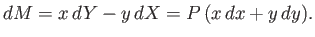
Figure 6.20:
Source in the presence of a rigid boundary.
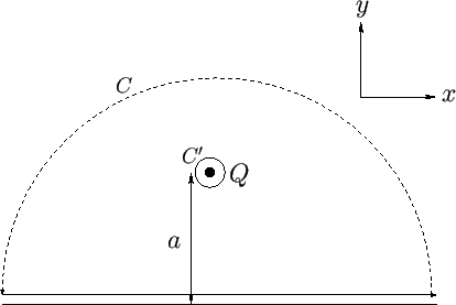 |
As an example of the use of the Blasius theorem, consider again the situation, discussed in Section 6.6, in which
a line source of strength  is located at
  ,
,  , and there is a rigid boundary at
  . As we
have seen, the complex velocity in the region
. As we
have seen, the complex velocity in the region  takes the form
 |
(6.189) |
Suppose that we evaluate the Blasius integral, (6.188), about the contour
shown in Figure 6.20. This
contour runs along the boundary, and is completed by a semi-circle in the upper half of the
-plane. As is easily demonstrated, in the limit in which the radius of the semi-circle tends to
infinity, the contribution of the curved section of the contour to the overall integral becomes negligible. In this case, only the straight
section of the contour contributes to the integral. Note that the straight section corresponds to a streamline (because it is
coincident with a rigid boundary). In other words, the contour
corresponds to a streamline at all constituent points that make a finite
contribution to the Blasius integral, which ensures that
is a valid contour for the application of the Blasius theorem. In fact, the Blasius integral
specifies the net force (per unit length) exerted on the whole fluid by the boundary. Observe, however, that the contour
can be deformed into the contour  , which takes the form of a small circle surrounding the source, without passing over
a singularity of
. (See Figure 6.20.) Hence, we can evaluate the Blasius integral around
without changing its value.
Thus,
, which takes the form of a small circle surrounding the source, without passing over
a singularity of
. (See Figure 6.20.) Hence, we can evaluate the Blasius integral around
without changing its value.
Thus,
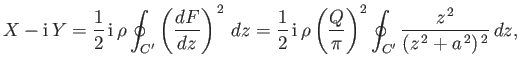 |
(6.190) |
or
![$\displaystyle X-{\rm i}\,Y = \frac{1}{8}\,{\rm i}\,\rho\left(\frac{Q}{\pi}\righ...
...}+\frac{2}{(z+{\rm i}\,a)\,(z-{\rm i}\,a)} + \frac{1}{(z+{\rm i}\,a)}\right]dz.$](img2416.png) |
(6.191) |
Writing
 ,
,
 , and
taking the limit
, and
taking the limit
 , we find that
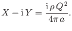 |
(6.192) |
In other words, the boundary exerts a force (per unit length)
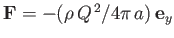 on the fluid. Hence, the
fluid exerts an equal and opposite force
on the fluid. Hence, the
fluid exerts an equal and opposite force
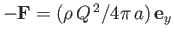 on the boundary. Of course, this
result is consistent with Equation (6.47). Incidentally, it is easily demonstrated from Equation (6.188) that there is zero
moment (about the
-axis) exerted on the boundary by the fluid, and vice versa.
on the boundary. Of course, this
result is consistent with Equation (6.47). Incidentally, it is easily demonstrated from Equation (6.188) that there is zero
moment (about the
-axis) exerted on the boundary by the fluid, and vice versa.
Consider a line source of strength
placed (at the origin) in a uniformly flowing fluid whose velocity is
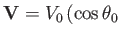 ,
,
 . From Section 6.4, the complex velocity potential of the net flow is
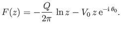 |
(6.193) |
The net force (per unit length) acting on the source (which is calculated by performing the Blasius integral around a large loop that follows
streamlines, and then shrinking the loop to a small circle centered on the source) is (see Exercise 1)
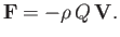 |
(6.194) |
This force acts in the opposite direction to the flow. Thus, an external force  , acting in the same
direction as the flow, must be applied to the source in order for it to remain stationary.
In fact, the previous result is valid even in a non-uniformly flowing fluid, as long as
, acting in the same
direction as the flow, must be applied to the source in order for it to remain stationary.
In fact, the previous result is valid even in a non-uniformly flowing fluid, as long as  is interpreted as the
fluid velocity at the location of the source (excluding the velocity field of the source itself).
is interpreted as the
fluid velocity at the location of the source (excluding the velocity field of the source itself).
Finally, consider a vortex filament of intensity
 placed at the origin in a uniformly flowing fluid whose velocity is
,
. From Section 6.4, the complex velocity potential of the net flow is
placed at the origin in a uniformly flowing fluid whose velocity is
,
. From Section 6.4, the complex velocity potential of the net flow is
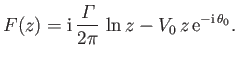 |
(6.195) |
The net force (per unit length) acting on the filament (which is calculated by performing the Blasius integral around a small circle centered on the filament) is (see Exercise 2)
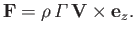 |
(6.196) |
This force is directed at right-angles to the direction of the flow (in the sense obtained by rotating
through
 in the opposite direction to the filament's direction of rotation).
Again, the previous result is valid even in a non-uniformly flowing fluid, as long as
is interpreted as the
fluid velocity at the location of the filament (excluding the velocity field of the filament itself).
in the opposite direction to the filament's direction of rotation).
Again, the previous result is valid even in a non-uniformly flowing fluid, as long as
is interpreted as the
fluid velocity at the location of the filament (excluding the velocity field of the filament itself).
Next: Exercises
Up: Two-Dimensional Potential Flow
Previous: Complex Line Integrals
Richard Fitzpatrick
2016-01-22