


Next: Method of Images
Up: Two-Dimensional Potential Flow
Previous: Complex Velocity Potential
Complex Velocity
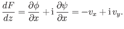
Equations (5.17), (5.20), and (6.15) imply that
 |
(6.35) |
Consequently,  is termed the complex velocity. It follows that
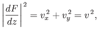 |
(6.36) |
where  is the flow speed.
A stagnation point is defined as a point in a flow pattern at which the flow speed,
, falls to zero. (See Section 5.8.)
According to the previous expression,
 |
(6.37) |
at a stagnation point. For instance, the stagnation points of the flow pattern produced when a cylindrical obstacle of radius  , centered on the origin, is placed in a uniform flow of speed
  , directed parallel to the
  -axis, and the circulation of the flow around is cylinder is
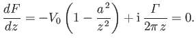
 , are found by setting the derivative of the complex potential (6.32) to zero.
It follows that the stagnation points satisfy the quadratic equation
, are found by setting the derivative of the complex potential (6.32) to zero.
It follows that the stagnation points satisfy the quadratic equation
 |
(6.38) |
The solutions are
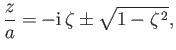 |
(6.39) |
where
 ,
with the proviso that
,
with the proviso that  , because the region
  is occupied by the cylinder. Thus, if
 then there are two stagnation points on the surface of the cylinder at
 and
and
 .
On the other hand, if
.
On the other hand, if  then there is a single stagnation point below the cylinder at
  and
and
 .
.
According to Section 4.15, Bernoulli's theorem in an steady, irrotational, incompressible fluid takes the form
 |
(6.40) |
where  is a uniform constant. Here, gravity (and any other body force) has been neglected. Thus, the
pressure distribution in such a fluid can be written
is a uniform constant. Here, gravity (and any other body force) has been neglected. Thus, the
pressure distribution in such a fluid can be written
 |
(6.41) |
Next: Method of Images
Up: Two-Dimensional Potential Flow
Previous: Complex Velocity Potential
Richard Fitzpatrick
2016-01-22