Spherical Coordinates

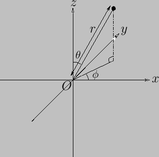
In the spherical coordinate system, $u_1=r$ , $u_2=\theta$ , and $u_3=\phi$ , where $r=\sqrt{x^{\,2}+y^{\,2}+z^{\,2}}$ , $\theta=\cos^{-1}(z/r)$ , $\phi=\tan^{-1}(y/x)$ , and $x$ , $y$ , $z$ are standard Cartesian coordinates. Thus, $r$ is the length of the radius vector, $\theta$ the angle subtended between the radius vector and the $z$ -axis, and $\phi$ the angle subtended between the projection of the radius vector onto the $x$ -$y$ plane and the $x$ -axis. (See Figure C.2.)

Figure C.2: Spherical coordinates.

A general vector ${\bf A}$ is written

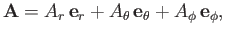$${\bf A} = A_r\,{\bf e}_r+ A_\theta\,{\bf e}_\theta + A_\phi\,{\bf e}_\phi,$$ (C.55)

where ${\bf e}_r=\nabla r/\vert\nabla r\vert$ , ${\bf e}_\theta = \nabla\theta/\vert\nabla\theta\vert$ , and ${\bf e}_\phi=\nabla \phi/\vert\nabla \phi\vert$ . Of course, the unit vectors ${\bf e}_r$ , ${\bf e}_\theta$ , and ${\bf e}_\phi$ are mutually orthogonal, so $A_r = {\bf A}\cdot {\bf e}_r$ , et cetera.

As is easily demonstrated, an element of length (squared) in the spherical coordinate system takes the form

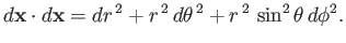$$d {\bf x}\cdot d{\bf x} = dr^{\,2} + r^{\,2}\,d\theta^{\,2} + r^{\,2}\,\sin^2\theta\,d\phi^2.$$ (C.56)

Hence, comparison with Equation (C.6) reveals that the scale factors for this system are

$$h_r = 1,$$ (C.57)

$$h_\theta = r,$$ (C.58)

$$h_\phi =r\,\sin\theta.$$ (C.59)

Thus, surface elements normal to ${\bf e}_r$ , ${\bf e}_\theta$ , and ${\bf e}_\phi$ are written

$$dS_r = r^{\,2}\,\sin\theta\,d\theta\,d\phi,$$ (C.60)

$$dS_\theta = r\,\sin\theta\,dr\,d\phi,$$ (C.61)

$$dS_\phi = r\,dr\,d\theta,$$ (C.62)

respectively, whereas a volume element takes the form

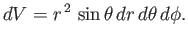$$dV = r^{\,2}\,\sin\theta\,dr\,d\theta\,d\phi.$$ (C.63)

According to Equations (C.13), (C.15), and (C.18), gradient, divergence, and curl in the spherical coordinate system are written

$$\nabla \psi = \frac{\partial \psi}{\partial r}\,{\bf e}_r + \frac{1}{r}\frac{... ...a + \frac{1}{r\,\sin\theta}\,\frac{\partial \psi}{\partial \phi}\,{\bf e}_\phi,$$ (C.64)

$$\nabla\cdot{\bf A} =\frac{1}{r^{\,2}}\,\frac{\partial}{\partial r}\,(r^{\,2}\,A_r) +... ...eta\,A_\theta)+ \frac{1}{r\,\sin\theta}\,\frac{\partial A_\phi}{\partial \phi},$$ (C.65)

$$\nabla\times {\bf A} = \left[\frac{1}{r\,\sin\theta}\,\frac{\partial}{\partial \theta}... ...frac{1}{r\,\sin\theta}\,\frac{\partial A_\theta}{\partial \phi}\right]{\bf e}_r$$

$$\phantom{=}+\left[\frac{1}{r\,\sin\theta}\,\frac{\partial A_r}{\p... ... \phi}-\frac{1}{r}\frac{\partial}{\partial r}\,(r\,A_\phi)\right]{\bf e}_\theta$$

$$\phantom{=}+ \left[\frac{1}{r}\,\frac{\partial}{\partial r}\,(r\,A_\theta) - \frac{1}{r}\,\frac{\partial A_r}{\partial\theta}\right]{\bf e}_\phi,\$$ (C.66)

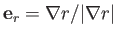
respectively. Here, $\psi({\bf r})$ is a general scalar field, and ${\bf A}({\bf r})$ a general vector field.

According to Equation (C.19), when expressed in spherical coordinates, the Laplacian of a scalar field becomes

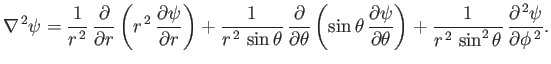$$\nabla^{\,2} \psi= \frac{1}{r^{\,2}}\,\frac{\partial}{\partial r}... ...rac{1}{r^{\,2}\,\sin^2\theta}\,\frac{\partial^{\,2} \psi}{\partial \phi^{\,2}}.$$ (C.67)

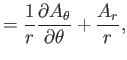
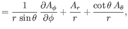
Moreover, from Equation (C.23), the components of $({\bf A}\cdot\nabla){\bf A}$ in the spherical coordinate system are

$$[({\bf A}\cdot\nabla)\,{\bf A}]_r ={\bf A}\cdot\nabla A_r - \frac{A_\theta^{\,2}+A_\phi^{\,2}}{r},$$ (C.68)

$$[({\bf A}\cdot\nabla)\,{\bf A}]_\theta = {\bf A}\cdot\nabla A_\theta + \frac{A_r\,A_\theta-\cot\theta\,A_\phi^{\,2}}{r},$$ (C.69)

$$[({\bf A}\cdot\nabla)\,{\bf A}]_\phi = {\bf A}\cdot\nabla A_\phi+ \frac{A_r\,A_\phi+\cot\theta\,A_\theta\,A_\phi}{r}.$$ (C.70)

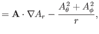
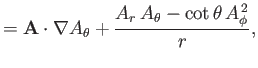
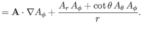
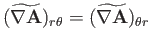
Now, according to Equation (C.26), the components of $\widetilde{\nabla {\bf A}}$ in the spherical coordinate system are

$$(\widetilde{\nabla {\bf A}})_{rr} = \frac{\partial A_r}{\partial r},$$ (C.71)

$$(\widetilde{\nabla {\bf A}})_{\theta\theta} =\frac{1}{r} \frac{\partial A_\theta}{\partial \theta}+ \frac{A_r}{r},$$ (C.72)

$$(\widetilde{\nabla {\bf A}})_{\phi\phi} =\frac{1}{r\,\sin\theta}\,\frac{\partial A_\phi}{\partial \phi}+ \frac{A_r}{r} + \frac{\cot\theta\,A_\theta}{r},$$ (C.73)

$$(\widetilde{\nabla {\bf A}})_{r\theta}=(\widetilde{\nabla {\bf A}})_{\theta r} = \frac{1}{2}\left(\frac{1}{r}\,\frac{\partial A_r}{\partial\theta} + \frac{\partial A_\theta}{\partial r} - \frac{A_\theta}{r}\right),$$ (C.74)

$$(\widetilde{\nabla {\bf A}})_{r\phi}=(\widetilde{\nabla {\bf A}})_{\phi r} =\frac{1}{2}\left(\frac{1}{r\,\sin\theta}\,\frac{\partial A_r}{\partial \phi} + \frac{\partial A_\phi}{\partial r}-\frac{A_\phi}{r}\right),$$ (C.75)

$$(\widetilde{\nabla {\bf A}})_{\theta \phi}=(\widetilde{\nabla {\bf A}})_{\phi\theta} =\frac{1}{2}\left(\frac{1}{r\,\sin\theta}\,\frac{\partial A_\thet... ...{r}\frac{\partial A_\phi}{\partial \theta}-\frac{\cot\theta\,A_\phi}{r}\right).$$ (C.76)

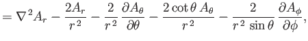
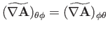
Finally, from Equation (C.28), the components of $\nabla^{\,2}{\bf A}$ in the spherical coordinate system are

$$(\nabla^{\,2}{\bf A})_r =\nabla^{\,2} A_r -\frac{2 A_r}{r^{\,2}}-\frac{2}{r^{\,2}}\,\frac... ...{r^{\,2}} -\frac{2}{r^{\,2}\,\sin\theta}\,\frac{\partial A_\phi}{\partial\phi},$$ (C.77)

$$(\nabla^{\,2}{\bf A})_\theta = \nabla^{\,2} A_\theta +\frac{2}{r^{\,2}}\,\frac{\partial A_r}{\... ...^2\theta} -\frac{2}{r^{\,2}\,\sin\theta}\,\frac{\partial A_\phi}{\partial\phi},$$ (C.78)

$$(\nabla^{\,2}{\bf A})_\phi =\nabla^{\,2} A_\phi-\frac{A_\phi}{r^{\,2}\,\sin^2\theta} + \frac... ...rac{2 \cot\theta}{r^{\,2}\,\sin\theta}\,\frac{\partial A_\theta}{\partial\phi}.$$ (C.79)