Next: Spherical Coordinates
Up: Non-Cartesian Coordinates
Previous: Orthogonal Curvilinear Coordinates
Cylindrical Coordinates
In the cylindrical coordinate system,  ,
,
 , and
, and  ,
where
,
where
 ,
,
 , and
, and  ,
,  ,
,  are standard Cartesian coordinates.
Thus,
are standard Cartesian coordinates.
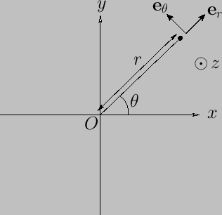
Thus,  is the perpendicular distance from the
-axis, and
is the perpendicular distance from the
-axis, and  the angle subtended between the projection of the radius vector (i.e., the vector connecting the origin to
a general point in space) onto the
-
plane and the
-axis. (See
Figure C.1.)
the angle subtended between the projection of the radius vector (i.e., the vector connecting the origin to
a general point in space) onto the
-
plane and the
-axis. (See
Figure C.1.)
Figure C.1:
Cylindrical coordinates.
 |
A general vector  is written
 |
(C.29) |
where
 ,
,
 , and
, and
 . Of course, the unit basis vectors
 ,
,
 , and
, and  are mutually orthogonal, so
 , et cetera.
As is easily demonstrated, an element of length (squared) in the cylindrical coordinate system takes the form
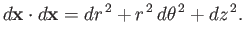 |
(C.30) |
Hence, comparison with Equation (C.6) reveals that the scale factors for this system are
Thus, surface elements normal to
,
, and
are
written
respectively, whereas
a
volume element takes the form
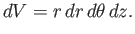 |
(C.37) |
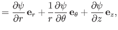
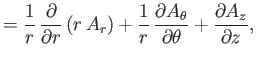
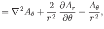
According to Equations (C.13), (C.15), and (C.18), gradient, divergence, and curl in the cylindrical
coordinate system are written
respectively. Here,
 is a general scalar field, and
 a general vector field.
According to Equation (C.19), when expressed in cylindrical coordinates, the Laplacian of a scalar field becomes
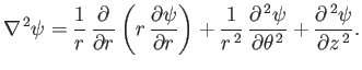 |
(C.41) |
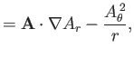
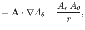
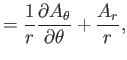
Moreover, from Equation (C.23), the components of
 in the cylindrical coordinate system are
Let us define the symmetric gradient tensor
![$\displaystyle \widetilde{\nabla {\bf A}} = \frac{1}{2}\left[\nabla {\bf A} + (\nabla{\bf A})^T\right].$](img7138.png) |
(C.45) |
Here, the superscript  denotes a transpose. Thus, if the
  element of some second-order tensor
  is
is  then the
corresponding element of
then the
corresponding element of  is
is  .
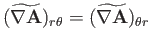
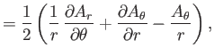
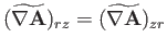
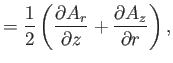
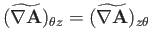
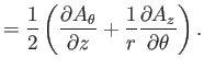
According to Equation (C.26), the components of
.
According to Equation (C.26), the components of
 in the cylindrical
coordinate system are
in the cylindrical
coordinate system are
 |
 |
(C.46) |
 |
 |
(C.47) |
 |
 |
(C.48) |
 |
 |
(C.49) |
 |
 |
(C.50) |
 |
 |
(C.51) |
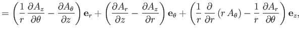
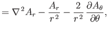
Finally, from Equation (C.28), the components of
 in the
cylindrical coordinate system are
in the
cylindrical coordinate system are
Next: Spherical Coordinates
Up: Non-Cartesian Coordinates
Previous: Orthogonal Curvilinear Coordinates
Richard Fitzpatrick
2016-01-22