Tensor Fields

We saw in Appendix A that a scalar field is a set of scalars associated with every point in space: for instance, $\phi({\bf x})$ , where ${\bf x}= (x_1,\,x_2,\,x_3)$ is a position vector. We also saw that a vector field is a set of vectors associated with every point in space: for instance, $a_i({\bf x})$ . It stands to reason, then, that a tensor field is a set of tensors associated with every point in space: for instance, $a_{ij}({\bf x})$ . It immediately follows that a scalar field is a zeroth-order tensor field, and a vector field is a first-order tensor field.

Most tensor fields encountered in physics are smoothly varying and differentiable. Consider the first-order tensor field $a_i({\bf x})$ . The various partial derivatives of the components of this field with respect to the Cartesian coordinates $x_i$ are written

$$\frac{\partial a_i}{\partial x_j}.$$ (B.50)

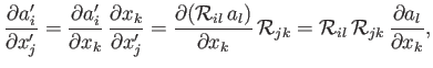
Moreover, this set of derivatives transform as the components of a second-order tensor. In order to demonstrate this, we need the transformation rule for the $x_i$ , which is the same as that for a first-order tensor: that is,

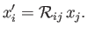$$x_i' = {\cal R}_{ij}\,x_j.$$ (B.51)

Thus,

$$\frac{\partial x_i'}{\partial x_j} = {\cal R}_{ij}.$$ (B.52)

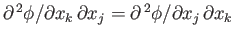
It is also easily shown that

$$\frac{\partial x_i}{\partial x_j'} = {\cal R}_{ji}.$$ (B.53)

Now,

$$\frac{\partial a_i'}{\partial x_j'} = \frac{\partial a_i'}{\parti... ...{\cal R}_{jk}= {\cal R}_{il}\,{\cal R}_{jk}\,\frac{\partial a_l}{\partial x_k},$$ (B.54)

which is the correct transformation rule for a second-order tensor. Here, use has been made of the chain rule, as well as Equation (B.53). [Note, from Equation (B.26), that the ${\cal R}_{ij}$ are not functions of position.] It follows, from the previous argument, that differentiating a tensor field increases its order by one: for instance, $\partial a_{ij}/\partial x_k$ is a third-order tensor. The only exception to this rule occurs when differentiation and contraction are combined. Thus, $\partial a_{ij}/\partial x_j$ is a first-order tensor, because it only contains a single free index.

The gradient (see Section A.18) of a scalar field is an example of a first-order tensor field (i.e., a vector field):

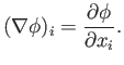$$(\nabla \phi)_i = \frac{\partial \phi}{\partial x_i}.$$ (B.55)

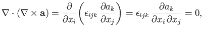
The divergence (see Section A.20) of a vector field is a contracted second-order tensor field that transforms as a scalar:

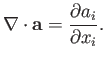$$\nabla\cdot {\bf a} = \frac{\partial a_i}{\partial x_i}.$$ (B.56)

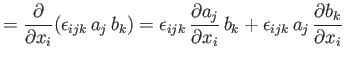
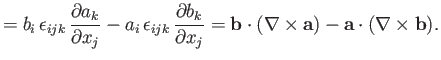
Finally, the curl (see Section A.22) of a vector field is a contracted fifth-order tensor that transforms as a vector

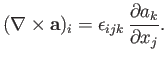$$(\nabla\times {\bf a})_i = \epsilon_{ijk}\,\frac{\partial a_k}{\partial x_j}.$$ (B.57)

The previous definitions can be used to prove a number of useful results. For instance,

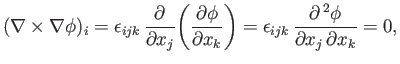$$(\nabla\times \nabla\phi)_i=\epsilon_{ijk}\,\frac{\partial }{\par... ...ight)= \epsilon_{ijk}\,\frac{\partial^{\,2}\phi}{\partial x_j\,\partial x_k}=0,$$ (B.58)

which follows from symmetry because $\epsilon_{ikj}=-\epsilon_{ijk}$ whereas $\partial^{\,2}\phi/\partial x_k\,\partial x_j = \partial^{\,2}\phi/\partial x_j\,\partial x_k$ . Likewise,

$$\nabla\cdot( \nabla\times {\bf a}) = \frac{\partial}{\partial x_i... ...j}\right)= \epsilon_{ijk}\,\frac{\partial a_k}{\partial x_i\,\partial x_j} = 0,$$ (B.59)

which again follows from symmetry. As a final example,

$$\nabla\cdot ({\bf a}\times {\bf b}) = \frac{\partial}{\partial x_i}\!\left(\epsilon_{ijk}\,a_j\,b_k\r... ..._j}{\partial x_i}\,b_k + \epsilon_{ijk}\,a_j\,\frac{\partial b_k}{\partial x_i}$$

$$=b_i\, \epsilon_{ijk}\,\frac{\partial a_k}{\partial x_j}-a_i\,\ep... ...x_j} ={\bf b}\cdot(\nabla \times {\bf a}) - {\bf a}\cdot(\nabla\times {\bf b}).$$ (B.60)

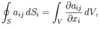
According to the divergence theorem (see Section A.20),

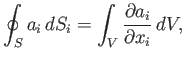$$\oint_S a_i\,dS_i = \int_V \frac{\partial a_i}{\partial x_i}\,dV,$$ (B.61)

where $S$ is a closed surface surrounding the volume $V$ . The previous theorem is easily generalized to give, for example,

$$\oint_S a_{ij}\,dS_i = \int_V \frac{\partial a_{ij}}{\partial x_i}\,dV,$$ (B.62)

or

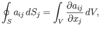$$\oint_S a_{ij}\,dS_j = \int_V \frac{\partial a_{ij}}{\partial x_j}\,dV,$$ (B.63)

or even

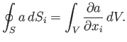$$\oint_S a\,dS_i = \int_V \frac{\partial a}{\partial x_i}\,dV.$$ (B.64)