Flow Around a Submerged Oblate Spheroid

Consider the conformal map

$$z+{\rm i}\,\varpi = c\,\sinh(\xi+{\rm i}\,\eta),$$ (7.115)

where $c$ is real and positive. It follows that

$$z = c\,\sinh\xi\,\cos\eta,$$ (7.116)

$$\varpi = c\,\cosh\xi\,\sin\eta.$$ (7.117)

Let

$$a =c\,\cosh\xi_0,$$ (7.118)

$$b =c\,\sinh\xi_0.$$ (7.119)

Thus, in the meridian plane, the curve $\xi=\xi_0$ corresponds to the ellipse

$$\left(\frac{\varpi}{a}\right)^2+\left(\frac{z}{b}\right)^2=1.$$ (7.120)

We conclude that the surface $\xi=\xi_0$ is an oblate spheroid (i.e., the three-dimensional surface obtained by rotating an ellipse about a minor axis) of major radius $a$ and minor radius $b$ . The constraints (7.87) and (7.90) yield

$$\psi(\xi\rightarrow\infty,\eta) = 0,$$ (7.121)

$$\psi(\xi_0,\eta) = -\frac{1}{2}\,V\,c^{\,2}\,\cosh^2\xi_0\,\sin^2\eta,$$ (7.122)

respectively. Setting $\psi(\xi,\eta)= F(\xi)\,\sin^2\eta$ , and substituting into the governing equation, (7.86), we obtain

$$\frac{d}{d\xi}\left(\frac{1}{\cosh\xi}\,\frac{dF}{d\xi}\right) - \frac{2}{\cosh\xi}\,F=0,$$ (7.123)

which can be rearranged to give

$$\frac{d}{d\xi}\left(\cosh\xi\,\frac{dF}{d\xi}-2\,\sinh\xi\,F\right)=0.$$ (7.124)

On integration, we get

$$\cosh\xi\,\frac{dF}{d\xi}-2\,\sinh\xi\,F = B,$$ (7.125)

which can be rearranged to give

$$\frac{d}{d\xi}\left(\frac{F}{\cosh^2\xi}\right)= \frac{B}{\cosh^3\xi}.$$ (7.126)

It follows that

$$F(\xi) =-B\,\cosh^2\xi \int_{\xi}^\infty \frac{d\xi'}{\cosh^3\xi'}$$

$$=-\frac{1}{2}\, B\,\cosh^2\xi\left[ \frac{\sinh\xi'}{\cosh^2\xi'}-\tan^{-1}\left(\frac{1}{\sinh\xi'}\right)\right]^{\infty}_{\xi}$$

$$= \frac{1}{2}\,B\left[\sinh\xi -\cosh^2\xi\,\tan^{-1}\left(\frac{1}{\sinh\xi}\right)\right],$$ (7.127)

where use has been made of the constraint (7.121). Let $e=(1-b^{\,2}/a^{\,2})^{1/2}$ be the eccentricity of the spheroid. Thus, $\cosh\xi_0=1/e$ , $\sinh\xi_0=(1-e^{\,2})^{1/2}/e$ , $c=e\,a$ , and $\tan^{-1}(1/\sinh\xi_0)=\sin^{-1}e$ . The constraint (7.122) yields

$$-\frac{1}{2}\,V\,a^{\,2} = F(\xi_0)= \frac{1}{2}\,B\left[\frac{(1-e^{\,2})^{1/2}}{e}-\frac{\sin^{-1}e}{e^{\,2}}\right],$$ (7.128)

or

$$B = - \left[\frac{V\,a^{\,2}\,e^{\,2}}{e\,(1-e^{\,2})^{1/2}-\sin^{-1}e}\right].$$ (7.129)

Hence,

$$\psi(\xi,\eta) =-\frac{1}{2}\,V\,a^{\,2}\,e^{\,2}\left[\frac{\sin... ...\xi\,\tan^{-1}(1/\sinh\xi)} {e\,(1-e^{\,2})^{1/2}-\sin^{-1}e}\right]\sin^2\eta.$$ (7.130)

Finally, from Equation (7.84),

$$\frac{\partial\phi}{\partial\eta} = -\frac{1}{c\,\cosh\xi\,\sin\eta}\,\frac{\partial\psi}{\partial\xi},$$ (7.131)

which can be integrated to give

$$\phi(\xi,\eta) =-V\,a\,e\left[\frac{1 -\sinh\xi\,\tan^{-1}(1/\sinh\xi)} {e\,(1-e^{\,2})^{1/2}-\sin^{-1}e}\right]\cos\eta.$$ (7.132)

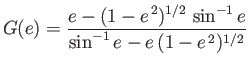
It is easily demonstrated that

$$\psi(\xi_0,\eta)= -\frac{1}{2}\,V\,a^{\,2}\,\sin^2\eta,$$ (7.133)

and

$$\phi(\xi_0,\eta) = V\,a\left[\frac{e-(1-e^{\,2})^{1/2}\,\sin^{-1} e}{\sin^{-1} e-e\,(1-e^{\,2})^{1/2}}\right]\cos\eta.$$ (7.134)

Thus,

$$K = -\pi\,\rho\left.\int_{\eta=0}^{\eta=\pi} \phi\,d\psi\right\ve... ...rac{e-(1-e^{\,2})^{1/2}\,\sin^{-1} e}{\sin^{-1} e-e\,(1-e^{\,2})^{1/2}}\right].$$ (7.135)

It follows that the added mass of the spheroid is

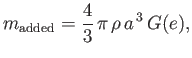$$m_{\rm added} = \frac{4}{3}\,\pi\,\rho\,a^{\,3}\,G(e),$$ (7.136)

where

$$G(e)= \frac{e-(1-e^{\,2})^{1/2}\,\sin^{-1} e}{\sin^{-1} e-e\,(1-e^{\,2})^{1/2}}$$ (7.137)

is a monotonic function that varies between $1/2$ when $e=0$ and $2/\pi$ when $e=1$ .

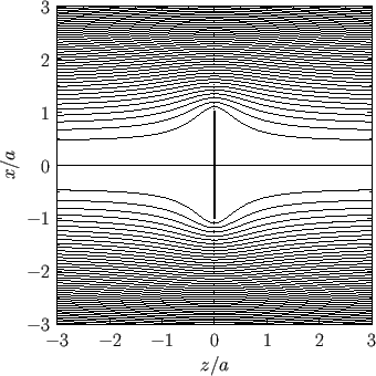
Figure: Contours of the Stokes stream function for the case of a disk of radius $a$ , lying in the $x$ -$y$ plane, and placed in a uniform, incompressible, irrotational flow directed parallel to the $z$ -axis.

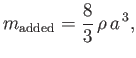
In the limit $e\rightarrow 1$ , our spheroid asymptotes to a thin disk of radius $a$ moving through the fluid in the direction perpendicular to its plane. Expressions (7.130), (7.132), and (7.136) yield

$$\psi(\xi,\eta) = -\frac{1}{2}\,V\,a^{\,2}\,\sin^2\eta,$$ (7.138)

$$\phi(\xi,\eta) = \frac{2}{\pi}\,V\,a\,\cos\eta,$$ (7.139)

and

$$m_{\rm added} = \frac{8}{3}\,\rho\,a^{\,3},$$ (7.140)

respectively. Here, $z=\sinh\xi\,\cos\eta$ and $\varpi=\cosh\xi\,\sin\eta$ . It follows that, in the instantaneous rest frame of the disk,

$$\psi(\varpi,z)=- \frac{1}{4}\,V\left[a^{\,2}+z^{\,2}+\varpi^{\,2}... ...rpi^{\,2})^2-4\,a^{\,2}\,\varpi^{\,2}}\,\right] + \frac{1}{2}\,V\,\varpi^{\,2}.$$ (7.141)

This flow pattern, which corresponds to that of a thin disk placed in a uniform flow perpendicular to its plane, is visualized in Figure 7.6.