Next: Flow Around a Submerged
Up: Axisymmetric Incompressible Inviscid Flow
Previous: Motion of a Submerged
As we saw in Section 6.7, conformal maps are extremely useful in the theory of two-dimensional, irrotational,
incompressible
flows. It turns out that such maps also have applications to the theory of axisymmetric, irrotational, incompressible flows.
Consider the general coordinate transformation
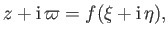 |
(7.79) |
where  is an analytic function. The Cauchy-Riemann relations (see Section 6.3) yield
It follows, from the previous two expressions, that
 . In other words,
  and
and  are orthogonal
coordinates in the meridian plane. [Incidentally, we are assuming that
are orthogonal
coordinates in the meridian plane. [Incidentally, we are assuming that
 are a right-handed set of coordinates.] Furthermore, it can also be shown from the Cauchy-Riemann relations that
![$\displaystyle h_\xi=h_\eta= \left[\left(\frac{\partial z}{\partial\xi}\right)^2...
...}\right)^2+ \left(\frac{\partial \varpi}{\partial\eta}\right)^2\right]^{\,1/2},$](img2690.png) |
(7.82) |
where
 and
and
 .
Writing the flow velocity in terms of a velocity potential, so that
.
Writing the flow velocity in terms of a velocity potential, so that
 , or, alternatively, in terms
of a Stokes stream function, so that
, or, alternatively, in terms
of a Stokes stream function, so that
 , we get
Of course, writing the velocity field in terms of a Stokes stream function ensures that the field is incompressible, which
also implies that
 . The additional requirement that the field be irrotational
yields
. The additional requirement that the field be irrotational
yields
 . Making use of the analysis of Appendix C, this requirement reduces to
 |
(7.85) |
or
 |
(7.86) |
Figure 7.5:
An axisymmetric solid body moving through an incompressible irrotational fluid.
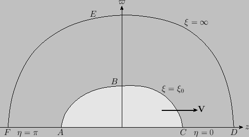 |
Let  represent the surface of an axisymmetric solid body moving with velocity
 through an
incompressible irrotational fluid that is at rest a long way from the body. Let the fluid occupy the region
through an
incompressible irrotational fluid that is at rest a long way from the body. Let the fluid occupy the region
 , where
 far from the body. (See Figure 7.5.) Let
be an angular coordinate such that
far from the body. (See Figure 7.5.) Let
be an angular coordinate such that  on
the positive
on
the positive  -axis, and
  on the negative
-axis. The fact that the fluid is at rest at infinity implies that
on the negative
-axis. The fact that the fluid is at rest at infinity implies that  asymptotes to
a constant a long way from the body. Without loss of generality, we can chose this constant to be zero. Thus, one constraint on the
system is that
asymptotes to
a constant a long way from the body. Without loss of generality, we can chose this constant to be zero. Thus, one constraint on the
system is that
 |
(7.87) |
The appropriate constraint at the surface of the body is that
 |
(7.88) |
where
 . However, we can write
 , where
 .
(See Section 7.6.) Hence, from Equation (7.83), the previous constraint becomes
.
(See Section 7.6.) Hence, from Equation (7.83), the previous constraint becomes
 |
(7.89) |
when
. Integrating, making use of the constraint (7.87) (which implies that  on the
-axis, where
is constant, by symmetry), we obtain
on the
-axis, where
is constant, by symmetry), we obtain
 |
(7.90) |
We can also set the velocity potential,  , to zero at infinity, and on the
-axis.
, to zero at infinity, and on the
-axis.
The total kinetic energy of the fluid surrounding the moving body is
 |
(7.91) |
where we have made use of the fact that
. Here,  is the fluid mass density, and
  is an element of the volume obtained by rotating the area
  , shown in Figure 7.5, about the
-axis. Making use of the divergence theorem, we obtain
, shown in Figure 7.5, about the
-axis. Making use of the divergence theorem, we obtain
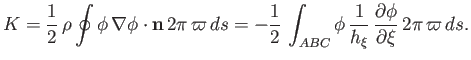 |
(7.92) |
where  is an element of the curve
, and
is an element of the curve
, and  is an outward pointing, unit, normal vector to the area
. Here, we have
made use of the fact that the velocity potential is zero at infinity (i.e., on
is an outward pointing, unit, normal vector to the area
. Here, we have
made use of the fact that the velocity potential is zero at infinity (i.e., on  ), and also on the
-axis (i.e., on
), and also on the
-axis (i.e., on  and
and  ).
On the curve
).
On the curve  , we can write
 . Furthermore, it follows from Equations (7.82) and (7.83)
that
. Furthermore, it follows from Equations (7.82) and (7.83)
that
 , and
, and
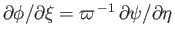 . Thus,
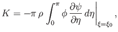 |
(7.93) |
or
 |
(7.94) |
As a simple example, consider the conformal map
 |
(7.95) |
where  is real and positive. It follows that
which implies that
 |
(7.98) |
where
 |
(7.99) |
Thus, the constant-
surfaces are concentric spheres of radius  . If we set
 |
(7.100) |
then the problem reduces to that of a sphere, of radius  , moving through a fluid that is at rest at infinity. This problem was solved, via different methods, in Section 7.10.
The constraints (7.87) and (7.90) yield
, moving through a fluid that is at rest at infinity. This problem was solved, via different methods, in Section 7.10.
The constraints (7.87) and (7.90) yield
where use has been made of Equation (7.97).
This suggests that we can write
 |
(7.103) |
Substitution into the governing equation, (7.86), gives
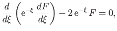 |
(7.104) |
whose most general solution is
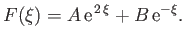 |
(7.105) |
The constraints (7.101) and (7.102) yield
respectively.
Thus, we obtain
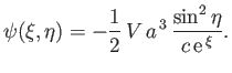 |
(7.108) |
Now, from Equations (7.84) and (7.97),
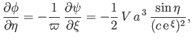 |
(7.109) |
which can be integrated to give
 |
(7.110) |
Note that the previous expression is formally the same as expression (7.63), as long as
we make the identifications
 ,
,
 , and
, and
 .
.
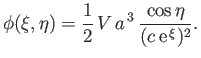
On the surface of the sphere,
, we obtain
Thus,
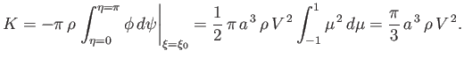 |
(7.113) |
As is clear from the analysis of Section 7.10, the sphere's added mass can be written
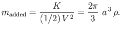 |
(7.114) |
Hence, we arrive at the standard result that the added mass is half the displaced mass [i.e., half of
 ].
].
Next: Flow Around a Submerged
Up: Axisymmetric Incompressible Inviscid Flow
Previous: Motion of a Submerged
Richard Fitzpatrick
2016-01-22