The Poincaré section

For the sake of definiteness, let us fix the normalized amplitude and frequency of the external drive to be $A=1.5$ and $\omega =2/3$, respectively.²⁴ Furthermore, let us investigate any changes which may develop in the nature of the pendulum's time-asymptotic motion as the quality-factor $Q$ is varied. Of course, if $Q$ is made sufficiently small (i.e., if the pendulum is embedded in a sufficiently viscous medium) then we expect the amplitude of the pendulum's time-asymptotic motion to become low enough that the linear analysis outlined in Sect. 4.2 remains valid. Indeed, we expect non-linear effects to manifest themselves as $Q$ is gradually made larger, and the amplitude of the pendulum's motion consequently increases to such an extent that the small angle approximation breaks down.

Figure 28: Equally spaced (in time) points on a time-asymptotic orbit in phase-space. Data calculated numerically for $Q=0.5$, $A=1.5$, $\omega =2/3$, $\theta (0)=0$, $v(0)=0$, and ${\tt Nacc} = 100$.

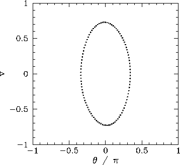Figure 28 shows a time-asymptotic orbit in phase-space calculated numerically for a case where $Q$ is sufficiently small (i.e., $Q=1/2$) that the small angle approximation holds reasonably well. Not surprisingly, the orbit is very similar to the analytic orbits described in Sect. 4.2. The fact that the orbit consists of a single loop, and forms a closed curve in phase-space, strongly suggests that the corresponding motion is periodic with the same period as the external drive--we term this type of motion period-1 motion. More generally, period-$n$ motion consists of motion which repeats itself exactly every $n$ periods of the external drive (and, obviously, does not repeat itself on any time-scale less than $n$ periods). Of course, period-1 motion is the only allowed time-asymptotic motion in the small angle limit.

It would certainly be helpful to possess a graphical test for period-$n$ motion. In fact, such a test was developed more than a hundred years ago by the French mathematician Henry Poincaré--nowadays, it is called a Poincaré section in his honour. The idea of a Poincaré section, as applied to a periodically driven pendulum, is very simple. As before, we calculate the time-asymptotic motion of the pendulum, and visualize it as a series of points in $\theta$-$v$ phase-space. However, we only plot one point per period of the external drive. To be more exact, we only plot a point when

$$\omega\,t = \phi + k\,2\pi$$ (97)

where $k$ is any integer, and $\phi$ is referred to as the Poincaré phase. For period-1 motion, in which the motion repeats itself exactly every period of the external drive, we expect the Poincaré section to consist of only one point in phase-space (i.e., we expect all of the points to plot on top of one another). Likewise, for period-2 motion, in which the motion repeats itself exactly every two periods of the external drive, we expect the Poincaré section to consist of two points in phase-space (i.e., we expect alternating points to plot on top of one another). Finally, for period-$n$ motion we expect the Poincaré section to consist of $n$ points in phase-space.

Figure 29: The Poincaré section of a time-asymptotic orbit. Data calculated numerically for $Q=0.5$, $A=1.5$, $\omega =2/3$, $\theta (0)=0$, $v(0)=0$, ${\tt Nacc} = 100$, and $\phi =0$.

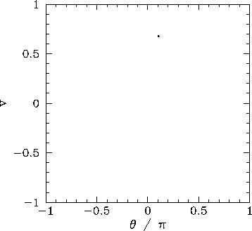Figure 29 displays the Poincaré section of the orbit shown in Fig. 28. The fact that the section consists of a single point confirms that the motion displayed in Fig. 28 is indeed period-1 motion.