


Next: The Poincaré section
Up: The chaotic pendulum
Previous: Numerical solution
Before proceeding with our investigation, we must first convince ourselves that
our numerical solutions are valid. Now, the usual
method of validating a numerical solution is to look for some special limits of the input parameters for
which analytic solutions are available, and then to test the numerical
solution in one of these limits against the associated analytic solution.
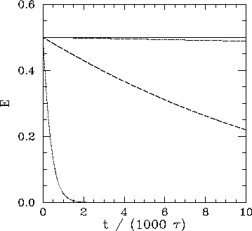
Figure 26:
The normalized energy  of an undamped, undriven,
pendulum versus time (measured in
natural periods of oscillation
of an undamped, undriven,
pendulum versus time (measured in
natural periods of oscillation  ). Data calculated numerically for
 ,
,  ,
,  ,
,  , and
, and  . The
dotted curve shows data for
. The
dotted curve shows data for  . The dashed curve
shows data for
. The dashed curve
shows data for
 . The dot-dashed curve
shows data for
. The dot-dashed curve
shows data for
 . Finally, the solid curve shows data
for
. Finally, the solid curve shows data
for
 .
.
 |
One special limit of
Eqs. (81) and (82) occurs when there is no viscous damping (i.e.,
 ) and no external driving (i.e.,
 ). In this case, we expect the
normalized energy of the pendulum
). In this case, we expect the
normalized energy of the pendulum
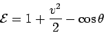 |
(94) |
to be a constant of the motion. Note that is defined such that the energy is
zero when the pendulum is in its stable equilibrium state (i.e., at rest, pointing
vertically downwards). Figure 26 shows versus time, calculated
numerically for an undamped, undriven, pendulum. Curves are plotted
for various values of the parameter Nacc, which, in this special case, measures the number
of time-steps taken by the integrator per (low amplitude) natural period of oscillation of the pendulum.
It can be seen that for  there is a strong spurious loss of energy, due
to truncation error in the numerical integration scheme, which eventually drains all
energy from the pendulum after about 2000 oscillations. For
there is a strong spurious loss of energy, due
to truncation error in the numerical integration scheme, which eventually drains all
energy from the pendulum after about 2000 oscillations. For  , the spurious
energy loss is less severe, but, nevertheless, still causes a more than 50% reduction in
pendulum energy after 10,000 oscillations. For
, the spurious
energy loss is less severe, but, nevertheless, still causes a more than 50% reduction in
pendulum energy after 10,000 oscillations. For  , the reduction in energy
after 10,000 oscillations is only about 1%. Finally, for
, the reduction in energy
after 10,000 oscillations is only about 1%. Finally, for  , the reduction in
energy after 10,000 oscillation is completely negligible. This test seems to indicate
that when
, the reduction in
energy after 10,000 oscillation is completely negligible. This test seems to indicate
that when
 our numerical solution describes the pendulum's
motion to
a high degree of precision for at least 10,000 oscillations.
our numerical solution describes the pendulum's
motion to
a high degree of precision for at least 10,000 oscillations.
Figure 27:
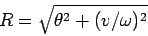
The parameter  associated with a linearized, damped, periodically
driven, pendulum versus time (measured in units of the period
of oscillation of the external drive). Data calculated numerically
for
associated with a linearized, damped, periodically
driven, pendulum versus time (measured in units of the period
of oscillation of the external drive). Data calculated numerically
for  ,
,  ,
,  , , and
  . The
dotted curve shows data for . The dashed curve
shows data for
. The solid curve
shows data for
.
. The
dotted curve shows data for . The dashed curve
shows data for
. The solid curve
shows data for
.
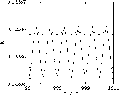 |
Another special limit of Eqs. (81) and (82) occurs when these equations
are linearized to give Eqs. (84) and (85). In this
case, we expect
 |
(95) |
to be a constant of the motion, after all transients have died away (see Sect. 4.2).
Figure 27 shows versus time, calculated numerically, for
a linearized, damped, periodically driven, pendulum. Curves are plotted
for various values of the parameter Nacc, which measures the number
of time-steps taken by the integrator per period of oscillation of the external drive.
As Nacc increases, it can be seen that the amplitude of the spurious oscillations in ,
which are due to truncation error in the numerical integration scheme, decreases rapidly.
Indeed, for
 these oscillations become effectively undetectable. According to
the analysis in Sect. 4.2, the parameter should take the value
these oscillations become effectively undetectable. According to
the analysis in Sect. 4.2, the parameter should take the value
 |
(96) |
Thus, for the case in hand (i.e.,
 ), we expect
  . It can be seen that
this prediction is borne out very accurately in Fig. 27. The above test essentially
confirms our previous conclusion that when
. It can be seen that
this prediction is borne out very accurately in Fig. 27. The above test essentially
confirms our previous conclusion that when
 our numerical solution
matches pendulum's actual motion to a high degree of
accuracy for many thousands of oscillation periods.
our numerical solution
matches pendulum's actual motion to a high degree of
accuracy for many thousands of oscillation periods.
Next: The Poincaré section
Up: The chaotic pendulum
Previous: Numerical solution
Richard Fitzpatrick
2006-03-29