Next: Analytic solution
Up: The chaotic pendulum
Previous: The chaotic pendulum
Up to now, we have mostly dealt with problems which are capable of analytic solution (so that we can
easily validate our numerical solutions). Let us now investigate a problem
which is quite intractable analytically, and in which meaningful progress can only be
made via numerical means.
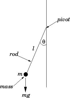
Consider a simple pendulum consisting of a point mass  , at the end of a light
rigid rod of length
, at the end of a light
rigid rod of length  , attached to a fixed frictionless pivot
which allows the rod (and the mass) to move freely under gravity in the vertical plane. Such a
pendulum is sketched in Fig. 21. Let us parameterize the instantaneous position
of the pendulum via the angle
, attached to a fixed frictionless pivot
which allows the rod (and the mass) to move freely under gravity in the vertical plane. Such a
pendulum is sketched in Fig. 21. Let us parameterize the instantaneous position
of the pendulum via the angle  the rod makes with the downward vertical. It is
assumed that the pendulum is free to swing through 360 degrees. Hence, and
the rod makes with the downward vertical. It is
assumed that the pendulum is free to swing through 360 degrees. Hence, and  both correspond to the same pendulum position.
The angular equation of motion of the pendulum is simply
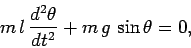 |
(72) |
where  is the downward acceleration due to gravity.
Suppose that the pendulum is embedded in a viscous medium (e.g., air).
Let us assume that the viscous drag torque acting on the pendulum is
governed by Stokes' law (see Sect. 3.12) and is, thus,
directly proportional to the pendulum's instantaneous velocity.
It follows that, in the presence of viscous drag, the above
equation generalizes to
is the downward acceleration due to gravity.
Suppose that the pendulum is embedded in a viscous medium (e.g., air).
Let us assume that the viscous drag torque acting on the pendulum is
governed by Stokes' law (see Sect. 3.12) and is, thus,
directly proportional to the pendulum's instantaneous velocity.
It follows that, in the presence of viscous drag, the above
equation generalizes to
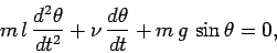 |
(73) |
where  is a positive constant parameterizing the viscosity of the medium
in question. Of course, viscous
damping will eventually drain all energy from the pendulum, leaving it in a stationary state.
In order to maintain the motion against viscosity, it is necessary to add some external driving.
For the sake of simplicity, we choose a fixed amplitude, periodic drive (which could arise, for
instance, via periodic oscillations of the pendulum's pivot point). Thus, the final equation
of motion of the pendulum is written
is a positive constant parameterizing the viscosity of the medium
in question. Of course, viscous
damping will eventually drain all energy from the pendulum, leaving it in a stationary state.
In order to maintain the motion against viscosity, it is necessary to add some external driving.
For the sake of simplicity, we choose a fixed amplitude, periodic drive (which could arise, for
instance, via periodic oscillations of the pendulum's pivot point). Thus, the final equation
of motion of the pendulum is written
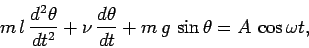 |
(74) |
where  and
and  are constants parameterizing the amplitude
and angular frequency of the external driving torque, respectively.
are constants parameterizing the amplitude
and angular frequency of the external driving torque, respectively.
Figure 21:
A simple pendulum.
 |
Let
 |
(75) |
Of course, we recognize  as the natural (angular) frequency of small
amplitude oscillations of the pendulum. We can conveniently normalize the
pendulum's equation of motion by writing,
as the natural (angular) frequency of small
amplitude oscillations of the pendulum. We can conveniently normalize the
pendulum's equation of motion by writing,
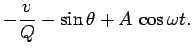
in which case Eq. (74) becomes
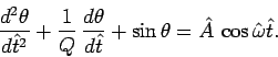 |
(80) |
From now on, the hats on normalized quantities will be omitted, for ease of
notation. Note that, in normalized units, the natural frequency of small amplitude
oscillations is unity. Moreover,  is the familiar quality-factor--roughly,
the number of oscillations of the undriven system which must
elapse before its energy is significantly
reduced via the action of viscosity. The quantity is the amplitude of the external
torque measured in units of the maximum possible gravitational torque. Finally,
is the angular frequency of the external torque measured in units of the
pendulum's natural frequency.
is the familiar quality-factor--roughly,
the number of oscillations of the undriven system which must
elapse before its energy is significantly
reduced via the action of viscosity. The quantity is the amplitude of the external
torque measured in units of the maximum possible gravitational torque. Finally,
is the angular frequency of the external torque measured in units of the
pendulum's natural frequency.
Equation (80) is clearly a second-order o.d.e. It can, therefore, also be written as
two coupled first-order o.d.e.s:
Next: Analytic solution
Up: The chaotic pendulum
Previous: The chaotic pendulum
Richard Fitzpatrick
2006-03-29