Sound Waves in Fluids
Consider a uniform fluid (at rest) whose equilibrium density and pressure
are  and
and  , respectively. Suppose that a sound wave propagates though the fluid, and that the density
and pressure perturbations produced by the wave are
, respectively. Suppose that a sound wave propagates though the fluid, and that the density
and pressure perturbations produced by the wave are
 and
and  , respectively. Incidentally, the quantity is
often referred to as the acoustic pressure. In two
dimensions (i.e., neglecting any variation of perturbed quantities in the
, respectively. Incidentally, the quantity is
often referred to as the acoustic pressure. In two
dimensions (i.e., neglecting any variation of perturbed quantities in the  -direction), the equations governing the propagation of
a sound wave though a uniform fluid are (Landau and Lifshitz 1959)
(See Section 9.12 for a more complete discussion of fluid equations.)
Here,
-direction), the equations governing the propagation of
a sound wave though a uniform fluid are (Landau and Lifshitz 1959)
(See Section 9.12 for a more complete discussion of fluid equations.)
Here,
 is the perturbation to the fluid velocity produced by the wave, and
 |
(7.194) |
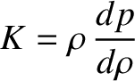
is the bulk modulus. The bulk modulus is a quantity with the units of
pressure that measures a given substance's resistance to uniform compression. The bulk modulus of an ideal
gas is  , where
  is the ratio of specific heats. On the other hand, the bulk modulus of
water at
is the ratio of specific heats. On the other hand, the bulk modulus of
water at
 is
is
 (Wikipedia contributors 2018).
It is helpful to write
where
 is conventionally referred to as a velocity potential.
It follows from Equations (7.192) and (7.193) that
is conventionally referred to as a velocity potential.
It follows from Equations (7.192) and (7.193) that
 |
(7.197) |
Moreover, substitution into Equation (7.194) yields the wave equation
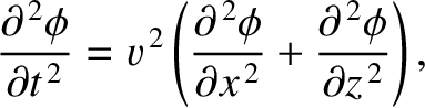 |
(7.198) |
where the characteristic wave speed is
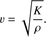 |
(7.199) |
For the case of an ideal gas, for which
 , we obtain
 . (See Section 5.4.) On the other hand, for
the case of water at
, for which
and
. (See Section 5.4.) On the other hand, for
the case of water at
, for which
and
 ,
we get
,
we get
 . This prediction is in good agreement with the measured sound speed in water
at
, which is
. This prediction is in good agreement with the measured sound speed in water
at
, which is
 (Wikipedia contributors 2018).
Forming the sum of  times Equation (7.192),
  times Equation (7.193), and
 times Equation (7.194), we obtain
 |
(7.200) |
where
Equation (7.201) can be recognized as a two-dimensional energy conservation equation. (See Section 6.5.)
Here,  is the acoustic energy density, and
 and
and
 are the acoustic energy fluxes
in the
are the acoustic energy fluxes
in the  - and
- and  -directions, respectively.
Consider a situation (analogous to that illustrated in Figure 7.7) in which a sound wave is incident at an
interface between two uniform immiscible fluids. Let the region  be occupied by a fluid of equilibrium density
  and sound speed
  , and let the region
  be occupied by a fluid of equilibrium density
  and
sound speed
and
sound speed  . We can write the wavevectors of the incident, reflected, and refracted waves as
respectively. Here, for the sake of simplicity, we have assumed that all three wavevectors lie in the same plane (as is
readily demonstrated; see Section 7.8.) Moreover, in order to be valid solutions of the wave equation, (7.199), all three waves must
satisfy the dispersion
relation
 , where
  is the common wave frequency. Finally,
  ,
,  , and
, and  are
the angles of incidence, reflection, and refraction, respectively. (See Section 7.8.)
are
the angles of incidence, reflection, and refraction, respectively. (See Section 7.8.)
The velocity potential in the region is written
where the first and second terms on the right-hand side specify the incident and reflected waves, respectively.
The velocity potential in the region takes the form
![$\displaystyle \phi(x,z,t) = \phi_t\,\cos[\omega\,(t-\sin\theta_t\,x/v_2-\cos\theta_t\,z/v_2)],$](img2266.png) |
(7.208) |
where the term on the right-hand side specifies the refracted wave.
The first physical matching constraint that must be satisfied at the interface is continuity of the acoustic pressure; that is,
![$\displaystyle [\tilde{p}]_{z=0_-}^{z=0_+}=-\left[\rho\,\frac{\partial\phi}{\partial t}\right]_{z=0_-}^{z=0_+}=0.$](img2267.png) |
(7.209) |
This contraint yields
The previous equation holds at all values of . This is only possible if
These two expressions are analogous to the laws of reflection and refraction, respectively, of geometric optics. (See Section 7.8.)
This suggests that these laws are of universal validity, rather than being restricted to light waves. Equation (7.211) reduces to
 |
(7.212) |
The second physical matching constraint that must be satisfied at the interface is continuity of the
normal velocity; that is,
![$\displaystyle [v_z]_{z=0_-}^{z=0_+} = \left[\frac{\partial\phi}{\partial z}\right]_{z=0_-}^{z=0_+} = 0.$](img2274.png) |
(7.213) |
This constraint yields
 |
(7.214) |
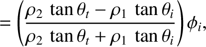
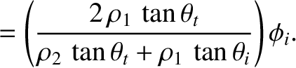
where use has been made of Equation (7.213). Equations (7.214) and (7.216) can be combined to give
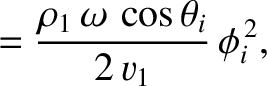
Equations (7.197), (7.198), and (7.204) reveal that the mean acoustic energy fluxes, normal
to the interface, associated with the incident, reflected, and refracted waves are
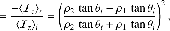
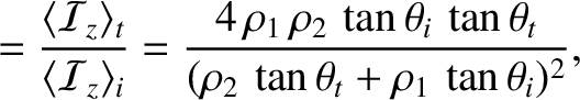
respectively. Thus, it follows that the coefficients of reflection and transmission at the interface
are
respectively. It is actually possible for there to be no reflection at the interface (i.e.,  ), provided that
 .
This criterion yields
.
This criterion yields
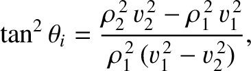 |
(7.222) |
which can only be satisfied if
 and
and  , or if
 and
and  .
The critical angle of incidence at which there is no reflection is sometimes called the angle of intromission.
However, not every pair of immiscible fluids possesses such an angle.
.
The critical angle of incidence at which there is no reflection is sometimes called the angle of intromission.
However, not every pair of immiscible fluids possesses such an angle.


![$\displaystyle = \phi_i\,\cos[\omega\,(t-\sin\theta_i\,x/v_1-\cos\theta_i\,z/v_1)]$](img2264.png)
![$\displaystyle ~~~~+\phi_r\,\cos[\omega\,(t-\sin\theta_r\,x/v_1+\cos\theta_r\,z/v_1)],$](img2265.png)


![\begin{multline}
\rho_1\,\omega\,\phi_i\,\sin[\omega\,(t-\sin\theta_i\,x/v_1)]+\...
...]
=\rho_2\,\omega\,\phi_t\,\sin[\omega\,(t-\sin\theta_t\,x/v_2)].
\end{multline}](img2268.png)