Fourier Analysis
Playing a musical instrument, such as a guitar or an organ, generates
a set of standing waves that cause a sympathetic oscillation in the surrounding air. Such an oscillation consists of a fundamental harmonic,
whose frequency determines the pitch of the musical note heard by the listener,
accompanied by a set of overtone harmonics that determine the timbre of the note. By definition, the oscillation frequencies of the overtone harmonics are
integer multiples of that of the fundamental.
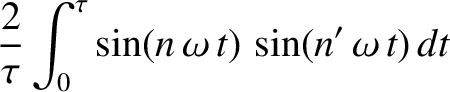
Thus, we expect the pressure perturbation generated in a listener's ear to have the general form
 |
(5.47) |
where  is the angular frequency of the fundamental (i.e.,
  ) harmonic, and the
  and
and  are the amplitudes and phases of the
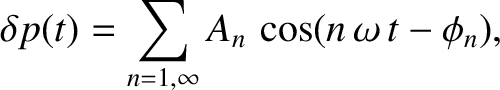
various harmonics. The preceding expression can also be written
are the amplitudes and phases of the
various harmonics. The preceding expression can also be written
![$\displaystyle \delta p(t) = \sum_{n=1,\infty} \left[C_{n}\,\cos(n\,\omega\,t)+ S_{n}\,\sin(n\,\omega\,t)\right],$](img1245.png) |
(5.48) |
where
 and
and
 . The function
 is
periodic in time with period
is
periodic in time with period
 . In other words,
 for all
  .
This follows because of the mathematical identities
.
This follows because of the mathematical identities
 and
and
 , where
  is an integer. [Moreover, there is no
 for which
 for all .]
Can any periodic waveform be represented as a linear superposition of sine and cosine waveforms, whose periods are integer subdivisions of that of the waveform, such as that specified in Equation (5.48)? To put it another way, given an arbitrary periodic
waveform
, can we uniquely determine the constants
for all .]
Can any periodic waveform be represented as a linear superposition of sine and cosine waveforms, whose periods are integer subdivisions of that of the waveform, such as that specified in Equation (5.48)? To put it another way, given an arbitrary periodic
waveform
, can we uniquely determine the constants  and
and  appearing in Equation (5.48)? It turns out that we can. Incidentally, the decomposition of
a periodic waveform into a linear superposition of sinusoidal waveforms is commonly known
as Fourier analysis.
appearing in Equation (5.48)? It turns out that we can. Incidentally, the decomposition of
a periodic waveform into a linear superposition of sinusoidal waveforms is commonly known
as Fourier analysis.
The problem under investigation is as follows. Given a periodic waveform  ,
where
,
where
 for all , we need to determine the constants and in the
expansion
for all , we need to determine the constants and in the
expansion
![$\displaystyle y(t) = \sum_{n'=1,\infty} \left[C_{n'}\,\cos(n'\,\omega\,t)+ S_{n'}\,\sin(n'\,\omega\,t)\right],$](img1258.png) |
(5.49) |
where
 |
(5.50) |
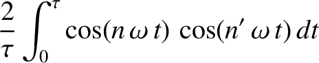
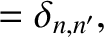
It can be demonstrated that [cf., Equation (4.53)]
where and  are positive integers. Thus, multiplying Equation (5.49) by
 , and then integrating over from 0 to
  , we obtain
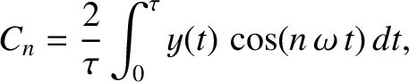 |
(5.54) |
where use has been made of Equation (5.51)–(5.53), as well as Equation (4.54). Likewise, multiplying
Equation (5.49) by
 , and then integrating over from 0 to , we obtain
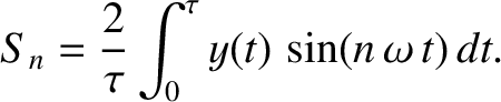 |
(5.55) |
Hence, we have uniquely determined the constants and in the expansion (5.49). These constants are generally known as
Fourier coefficients,
whereas the expansion itself is known
as either a Fourier expansion or a Fourier series.
Figure 5.6:
Fourier reconstruction of a periodic sawtooth waveform. The top-left, top-right,
bottom-left, and bottom-right panels correspond to reconstructions using 4, 8, 32, and 64 terms, respectively, in the Fourier series.
|
|
In principle, there is no restriction on the waveform in the previous analysis, other
than the requirement that it be periodic in time. In other words, we ought to be able
to Fourier analyze any periodic waveform. Let us see how this works. Consider
the periodic sawtooth waveform
with
for all . See Figure 5.6. This waveform rises linearly from an initial
value  at
at  to a final value
  at
at  , discontinuously jumps
back to its initial value, and then repeats ad infinitum.
According to Equations (5.54) and
(5.55), the Fourier harmonics of the waveform are
where
, discontinuously jumps
back to its initial value, and then repeats ad infinitum.
According to Equations (5.54) and
(5.55), the Fourier harmonics of the waveform are
where
 .
Integration by parts (Riley 1974) yields
Hence, the Fourier reconstruction of the waveform is written
.
Integration by parts (Riley 1974) yields
Hence, the Fourier reconstruction of the waveform is written
 |
(5.61) |
Given that the Fourier coefficients fall off like  , as increases, it seems plausible that the preceding
series can be truncated after a finite number of terms without unduly affecting the reconstructed waveform. Figure 5.6 shows
the result of truncating the series after 4, 8, 16, and 32 terms. It can be seen that the reconstruction
becomes increasingly accurate as the number of terms retained in the series increases.
The annoying oscillations in the reconstructed waveform at , , and
, as increases, it seems plausible that the preceding
series can be truncated after a finite number of terms without unduly affecting the reconstructed waveform. Figure 5.6 shows
the result of truncating the series after 4, 8, 16, and 32 terms. It can be seen that the reconstruction
becomes increasingly accurate as the number of terms retained in the series increases.
The annoying oscillations in the reconstructed waveform at , , and  are
known as Gibbs' phenomena, and are the inevitable consequence of trying
to represent a discontinuous waveform as a Fourier series (Riley 1974). In fact, it can be demonstrated
mathematically that, no matter how many terms are retained in the series, the Gibbs'
phenomena never entirely go away (Zygmund 1955).
are
known as Gibbs' phenomena, and are the inevitable consequence of trying
to represent a discontinuous waveform as a Fourier series (Riley 1974). In fact, it can be demonstrated
mathematically that, no matter how many terms are retained in the series, the Gibbs'
phenomena never entirely go away (Zygmund 1955).
We can slightly generalize the Fourier series (5.49) by including an  term. In other words,
![$\displaystyle y(t) = C_0+ \sum_{n'=1,\infty} \left[C_{n'}\,\cos(n'\,\omega\,t)+ S_{n'}\,\sin(n'\,\omega\,t)\right],$](img1282.png) |
(5.62) |
which allows the waveform to have a non-zero average.
There is no term involving  , because
 when .
It can be demonstrated that
where
when .
It can be demonstrated that
where
 , and is a positive integer. Making use of the preceding expressions, as
well as Equations (5.51)–(5.53), we can show that
, and is a positive integer. Making use of the preceding expressions, as
well as Equations (5.51)–(5.53), we can show that
 |
(5.65) |
and also that Equations (5.54) and (5.55) still hold for  .
.
Figure 5.7:
Fourier reconstruction of a periodic “tent” waveform. The top-left, top-right,
bottom-left, and bottom-right panels correspond to reconstruction using the first 1, 2, 4, and 8
terms, respectively, in the Fourier series (in addition to the  term).
|
|
As an example, consider the periodic “tent” waveform
![\begin{displaymath}y(t) = 2\,A\left\{
\begin{array}{lcl}
t/\tau&\mbox{\hspace{0....
...1/2\\ [0.5ex]
1-t/\tau &&1/2< t/\tau \leq 1
\end{array}\right.,\end{displaymath}](img1291.png) |
(5.66) |
where
for all . See Figure 5.7. This waveform rises linearly from zero at , reaches a peak value  at
at  , falls
linearly, becomes zero again at , and repeats
ad infinitum. Moreover, the waveform has a non-zero average.
It can be demonstrated, from Equations (5.54), (5.55), (5.65), and (5.66), that
, falls
linearly, becomes zero again at , and repeats
ad infinitum. Moreover, the waveform has a non-zero average.
It can be demonstrated, from Equations (5.54), (5.55), (5.65), and (5.66), that
 |
(5.67) |
and
 |
(5.68) |
for  , with
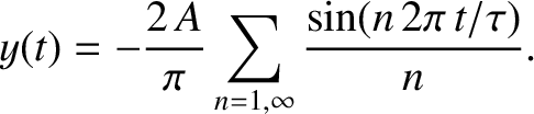
  for . In fact, only the odd- Fourier harmonics
are non-zero. Thus,
for . In fact, only the odd- Fourier harmonics
are non-zero. Thus,
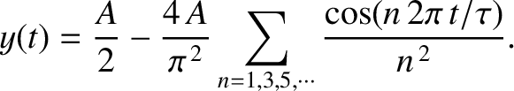 |
(5.69) |
Figure 5.7 shows
a Fourier reconstruction of the “tent” waveform using the first 1, 2, 4, and 8 terms (in addition to the term) in the Fourier series The reconstruction
becomes increasingly accurate as the number of terms in the series increases.
Moreover, in this example, there is no sign of Gibbs' phenomena,
because the tent waveform is completely continuous.
In our first example—that is, the sawtooth waveform—all of the
Fourier coefficients are zero, whereas in our second example—that is, the
tent waveform—all of the coefficients are zero. This occurs because the sawtooth waveform is odd in —that is,
 for all —whereas the tent waveform is even—that is,
 for all . It is a general rule that waveforms that are even in only
have cosines in their Fourier series, whereas waveforms that are odd only have sines (Riley1974). Waveforms
that are neither even nor odd in have both cosines and sines in their Fourier
series.
for all . It is a general rule that waveforms that are even in only
have cosines in their Fourier series, whereas waveforms that are odd only have sines (Riley1974). Waveforms
that are neither even nor odd in have both cosines and sines in their Fourier
series.
Fourier series arise quite naturally in the theory of standing waves, because the normal
modes of oscillation of any uniform continuous system possessing linear equations of motion
(e.g., a uniform string, an elastic rod, an ideal gas) take the form of spatial cosine and
sine waves whose wavelengths are rational fractions of one another. Thus, the instantaneous spatial waveform of such a system can always
be represented as a linear superposition of cosine and sine waves; that is, a Fourier
series in space, rather than in time. In fact, the
process of determining the amplitudes and phases of the normal modes of oscillation
from the
initial conditions is essentially equivalent to Fourier analyzing the initial conditions
in space. (See Sections 4.4 and 5.3.)
![\includegraphics[width=1\textwidth]{Chapter05/fig5_06.eps}](img1268.png)


![\includegraphics[width=1\textwidth]{Chapter05/fig5_07.eps}](img1290.png)