Birefringence
Up until now, our treatment of electromagnetic wave propagation through transparent dielectrics has been restricted to isotropic media in which the refractive index is independent
of either the direction of propagation or the polarization of the wave. However, there exists a
certain class of optically anisotropic materials (e.g., crystals with non-cubic lattices, and plastics under mechanical
stress) which are such that the refractive index varies with both the direction of propagation and the polarization. Such materials are said to be birefringent. Let us investigate the propagation of
electromagnetic waves through birefringent media.
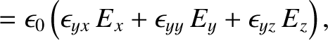
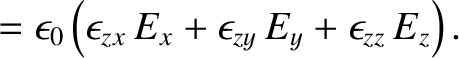
In a birefringent medium, the constitutive relation (7.53) generalizes to give
 |
(7.136) |
Here,  is the electric field-strength,
 the electric
displacement,
the electric
displacement,  the electric dipole moment per unit volume, and
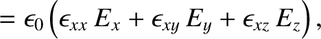
 is termed the dielectric tensor. In a general Cartesian coordinate
system, the dielectric tensor takes the form of a real 3 by 3 matrix. (However, the components
of this matrix transform under rotation of the coordinate axes in an analogous manner to that in which the components of a vector transform.) Thus, in component form, the previous equation
becomes
Note that
is termed the dielectric tensor. In a general Cartesian coordinate
system, the dielectric tensor takes the form of a real 3 by 3 matrix. (However, the components
of this matrix transform under rotation of the coordinate axes in an analogous manner to that in which the components of a vector transform.) Thus, in component form, the previous equation
becomes
Note that
 ,
,
 , and
, and
 (i.e., the dielectric tensor is symmetric) in a lossless birefringent medium (i.e., one that does not absorb wave energy).
Furthermore, the
(i.e., the dielectric tensor is symmetric) in a lossless birefringent medium (i.e., one that does not absorb wave energy).
Furthermore, the  and vectors are not necessarily parallel to one another in such
a medium.
and vectors are not necessarily parallel to one another in such
a medium.
It is a well-known fact that it is always possible to find a particular orientation of the Cartesian coordinate
axes that diagonalizes a symmetric tensor (Riley 1974). For the case of the dielectric tensor, these
special axes are called the principal axes of the dielectric medium in question. When the Cartesian axes are
aligned along the principal axes, the dielectric tensor takes the form
![\begin{displaymath}\bm{\epsilon} = \left(
\begin{array}{ccc}
\epsilon_{xx},&0,&0...
...psilon_{yy},&0\\ [0.5ex]
0,&0,&\epsilon_{zz}\end{array}\right).\end{displaymath}](img2111.png) |
(7.140) |
Here,
 ,
,
 , and
, and
 are known as the principal values
of the dielectric tensor. If the principal values are all equal to one another then the medium is termed isotropic.
If one of the principal values is different from the other two then the medium is termed monaxial. This nomenclature arises because the medium possesses a single optic axis (i.e., a direction of wave
propagation in which the phase velocity is independent of the wave polarization). Finally, if all
of the principal values are different from one another then the medium is termed biaxial (because it
possesses two optic axes). (Obviously, an isotropic medium possesses an infinite number of
optic axes corresponding to all the possible directions of wave propagation.)
are known as the principal values
of the dielectric tensor. If the principal values are all equal to one another then the medium is termed isotropic.
If one of the principal values is different from the other two then the medium is termed monaxial. This nomenclature arises because the medium possesses a single optic axis (i.e., a direction of wave
propagation in which the phase velocity is independent of the wave polarization). Finally, if all
of the principal values are different from one another then the medium is termed biaxial (because it
possesses two optic axes). (Obviously, an isotropic medium possesses an infinite number of
optic axes corresponding to all the possible directions of wave propagation.)
The equations that govern electromagnetic wave propagation through dielectric
media can be written (see Appendix C)
where
 . Here,
  is the magnetic field-strength, and
  the
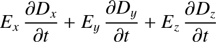
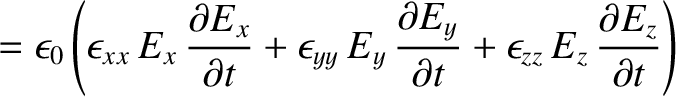
magnetic intensity. Taking
the
magnetic intensity. Taking  times Equation (7.142) plus
  times Equation (7.143)
plus
times Equation (7.143)
plus
 times Equation (7.144) plus
  times Equation (7.145) plus
  times
Equation (7.146) plus
times
Equation (7.146) plus  times Equation (7.147), and rearranging, we obtain
| 0 |
 |
|
| |
 |
(7.147) |
 |
(7.149) |
Hence, Equation (7.148) reduces to
 |
(7.150) |
where
We can recognize Equation (7.151) as a three-dimensional generalization of the
energy conservation equation (6.125). It follows that  is the electromagnetic
energy density (i.e., the electromagnetic energy per unit volume), whereas
is the electromagnetic
energy density (i.e., the electromagnetic energy per unit volume), whereas
 is the electromagnetic energy flux (i.e.,
electromagnetic energy flows at the rate
is the electromagnetic energy flux (i.e.,
electromagnetic energy flows at the rate
 joules per unit area per unit time in the direction of the
vector
).
joules per unit area per unit time in the direction of the
vector
).
Let us search for wave-like solutions of Equations (7.142)–(7.147) of the form
with
. Here, the wavevector is
 , and the
phase velocity is
, and the
phase velocity is
 , where
  is a unit vector.
Equations (7.142)–(7.144) yield
is a unit vector.
Equations (7.142)–(7.144) yield
 |
(7.156) |
whereas Equations (7.145)–(7.147) give
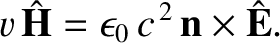 |
(7.157) |
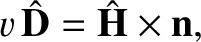
The previous two equations immediately imply that
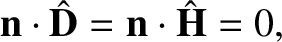 |
(7.158) |
and
 |
(7.159) |
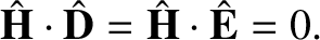
In other words, the electric displacement and the magnetic intensity are both perpendicular to
the wavevector. Furthermore, the magnetic intensity is perpendicular to both the electric displacement and
the electric field-strength.
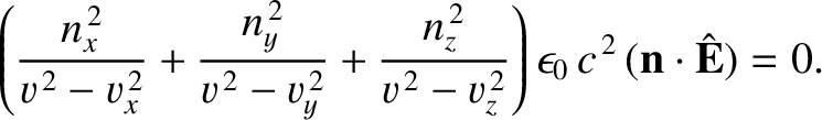
Equations (7.157) and (7.158) can also be combined to give
![$\displaystyle v^{\,2}\,\hat{\bf D} = \epsilon_0\,c^{\,2}\left[\hat{\bf E} - ({\bf n}\cdot\hat{\bf E})\,{\bf n}\right],$](img2157.png) |
(7.160) |
where use has been made of a standard vector identity.
The quantities
 ,
,
 , and
, and
 ,
where
,
,
are the principal components of the dielectric
tensor, are termed the principal velocities of the dielectric medium in question.
Now, given that
,
where
,
,
are the principal components of the dielectric
tensor, are termed the principal velocities of the dielectric medium in question.
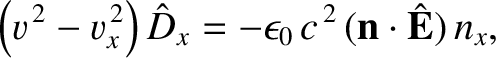
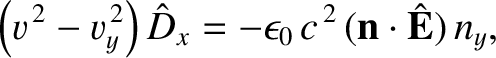
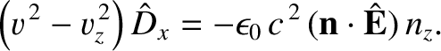
Now, given that
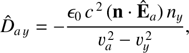
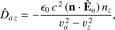
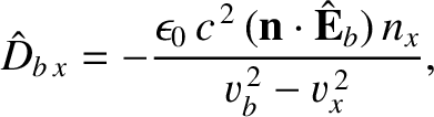
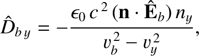
 , et cetera,
when the Cartesian axes are aligned along the principal axes, the three Cartesian components of the
previous equation can be written
Finally, because [see Equation (7.159)]
, et cetera,
when the Cartesian axes are aligned along the principal axes, the three Cartesian components of the
previous equation can be written
Finally, because [see Equation (7.159)]
 |
(7.164) |
we obtain
 |
(7.165) |
Assuming that
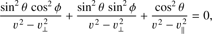
 , the previous equation yields
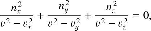 |
(7.166) |
which is known as the Fresnel equation.
The Fresnel equation is a quadratic equation for  that specifies the phase speeds,
  , of the two
independent electromagnetic wave polarizations that can propagate through a birefringent
medium in a particular direction, . In general, these two speeds are different. Let
, of the two
independent electromagnetic wave polarizations that can propagate through a birefringent
medium in a particular direction, . In general, these two speeds are different. Let  be the first speed,
 the associated electric displacement, and
 the associated electric field-strength. Likewise,
let
the associated electric field-strength. Likewise,
let  be the second speed,
 the associated electric displacement, and
 the associated electric field-strength
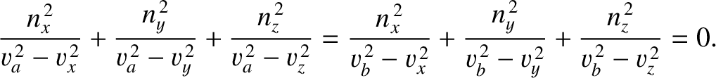
It follows from Equations (7.162)–(7.164) that
the associated electric field-strength
It follows from Equations (7.162)–(7.164) that
Hence,
However, according to the Fresnel equation, (7.167),
 |
(7.174) |
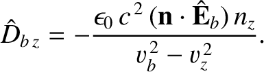
Hence, we deduce that
 |
(7.175) |
In other words, the two independent wave polarizations have mutually orthogonal electric displacements.
As an example, consider the propagation of an electromagnetic wave through a monaxial
material whose principal velocities are
 and
and
 , where
 . The corresponding principal
components of the dielectric tensor are
. The corresponding principal
components of the dielectric tensor are
 and
and
 . Of course,
 and
and
 In this case, the optic axis corresponds to the
  -axis. It is
convenient to specify the direction of wave propagation in terms of standard spherical
angles,
-axis. It is
convenient to specify the direction of wave propagation in terms of standard spherical
angles,
 |
(7.176) |
In particular,  is the angle subtended between the direction of wave propagation and
the optic axis.
is the angle subtended between the direction of wave propagation and
the optic axis.
The two independent electromagnetic wave polarizations that can propagate through a
monaxial material are termed the ordinary wave and the extraordinary wave.
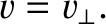
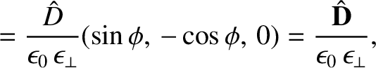
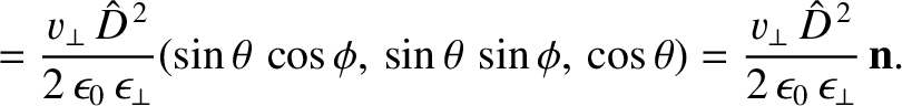
The ordinary wave is such that
 , which is
one way of satisfying Equation (7.166). Assuming that the Cartesian axes correspond to the
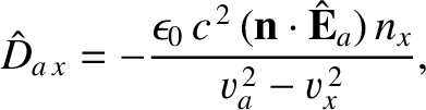
principal axes, it is easily demonstrated that
, which is
one way of satisfying Equation (7.166). Assuming that the Cartesian axes correspond to the
principal axes, it is easily demonstrated that
Here,
 denotes an average over a wave period.
Substitution of Equations (7.178) and (7.179) into Equation (7.161)
reveals that
denotes an average over a wave period.
Substitution of Equations (7.178) and (7.179) into Equation (7.161)
reveals that
 |
(7.181) |
In other words, the ordinary wave propagates at the fixed phase speed  , irrespective
of its direction of propagation. Furthermore, the electric field-strength is parallel to the electric
displacement, and the electromagnetic energy flux is parallel to the wavevector.
, irrespective
of its direction of propagation. Furthermore, the electric field-strength is parallel to the electric
displacement, and the electromagnetic energy flux is parallel to the wavevector.
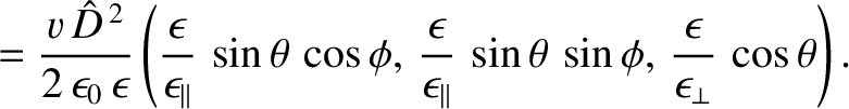
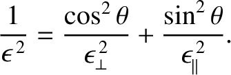
The phase speed of the extraordinary wave is obtained directly from the Fresnel equation,
(7.167), which yields
 |
(7.182) |
or
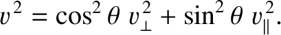 |
(7.183) |
It follows that the phase speed of the extraordinary wave varies with its direction of propagation.
The phase speed matches that of the ordinary wave when the wave propagates along the
optic axis (i.e., when  ); otherwise, it is different.
It is easily demonstrated that
); otherwise, it is different.
It is easily demonstrated that
 |
 |
(7.184) |
 |
 |
(7.185) |
 |
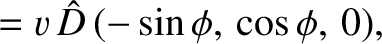 |
(7.186) |
 |
 |
(7.187) |
 |
(7.188) |
It can be seen that the
 and
and
 vectors are not parallel to one another.
Moreover, the electromagnetic energy flux is not parallel to the wavevector. If
vectors are not parallel to one another.
Moreover, the electromagnetic energy flux is not parallel to the wavevector. If  is the angle subtended between the directions of the
and
vectors then
is the angle subtended between the directions of the
and
vectors then
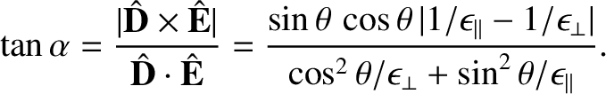 |
(7.189) |
Likewise, if  is the angle subtended between the directions of the electromagnetic
energy flux and the wavevector then
is the angle subtended between the directions of the electromagnetic
energy flux and the wavevector then
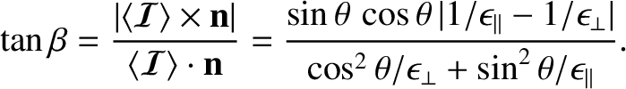 |
(7.190) |
It follows that
 . Moreover, these two angles are only zero when the extraordinary wave propagates
parallel (i.e.,
. Moreover, these two angles are only zero when the extraordinary wave propagates
parallel (i.e.,
 ) or perpendicular (i.e.,
 ) to the optic axis.
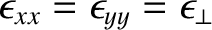
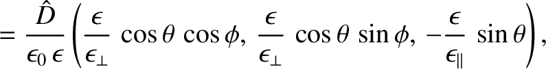
Figure 7.13:
Birefringence.
|
|
Figure 7.13 illustrates what happens when unpolarized light is normally incident on a
slab of birefringent material in such a manner that the incident light is neither parallel nor
perpendicular to the optic axis. Because of the normal incidence, the wavevectors of both
the ordinary and the extraordinary rays are not refracted, and remain parallel to the direction of incidence. However, the
ray path is actually coincident with the associated electromagnetic energy flux. For the
ordinary ray, the electromagnetic energy flux is parallel to the wavevector. However, for
the extraordinary ray, the electromagnetic energy flux subtends a finite angle with the wavevector.
Consequently, although the ordinary ray passes through the slab without changing direction, the direction
of the extraordinary ray suffers a sideways deviation. This type of double refraction is known as
birefringence.


![$\displaystyle = \hat{\bf E}\,\cos\left[k\,(v\,t-{\bf n}\cdot{\bf r})\right],$](img2146.png)
![$\displaystyle = \hat{\bf D}\,\cos\left[k\,(v\,t-{\bf n}\cdot{\bf r})\right],$](img2148.png)
![$\displaystyle = \hat{\bf H}\,\cos\left[k\,(v\,t-{\bf n}\cdot{\bf r})\right],$](img2150.png)


![\includegraphics[width=0.9\textwidth]{Chapter07/fig7_13.eps}](img2221.png)