Diffraction from Circular Aperture
Consider the diffraction pattern of a circular aperture of radius  whose center lies
at
whose center lies
at  . (See Section 10.10.) We expect the pattern to be rotationally symmetric about the
  -axis. In other words, we expect
the intensity of the illumination on the projection screen to be only a function of the
radial coordinate
-axis. In other words, we expect
the intensity of the illumination on the projection screen to be only a function of the
radial coordinate
 . It is helpful to redefine the dimensionless parameters
 and
and  as follows:
Thus, now parameterizes the aperture radius, whereas is a normalized radial
coordinate on the projection screen. Note, from Equation (10.96), that the far-field limit
corresponds to
as follows:
Thus, now parameterizes the aperture radius, whereas is a normalized radial
coordinate on the projection screen. Note, from Equation (10.96), that the far-field limit
corresponds to
 , whereas the near-field limit corresponds to
  .
Furthermore, a point on the projection screen lies in the
geometric (i.e., as predicted by geometric optics) lit part of the screen if
.
Furthermore, a point on the projection screen lies in the
geometric (i.e., as predicted by geometric optics) lit part of the screen if  ,
and vice versa. Finally, the aperture function takes the form
,
and vice versa. Finally, the aperture function takes the form
![\begin{displaymath}f(v) = \left\{
\begin{array}{lll}
1&\mbox{\hspace{0.5cm}}& \mbox{$v<u$\ }\\ [0.5ex]
0&&\mbox{otherwise}\end{array}\right..\end{displaymath}](img3677.png) |
(10.141) |
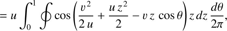
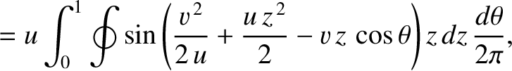
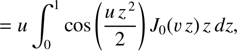
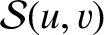
When expressed in terms of the new variables, Equations (10.103) and (10.104) transform to give
where
 .
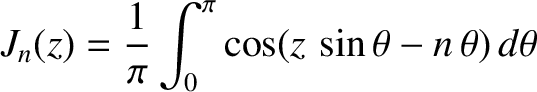
Now, (Abramowitz and Stegun 1965)
where (ibid.)
.
Now, (Abramowitz and Stegun 1965)
where (ibid.)
 |
(10.146) |
denotes a Bessel function of degree  .
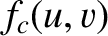
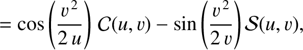
Hence, making use of some trigonometric identities (see Appendix B),
Equations (10.142) and (10.143) reduce to
where
.
Hence, making use of some trigonometric identities (see Appendix B),
Equations (10.142) and (10.143) reduce to
where
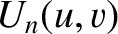
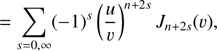
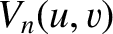
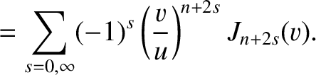
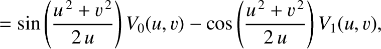
It is helpful, at this stage, to introduce the so-called Lommel functions (of two arguments) (Watson 1962)
In the geometric lit region, , the integrals
 and
and
 are conveniently expanded in terms of the convergent
  Lommel functions (Born and Wolf 1980)
(See Exercise 22.)
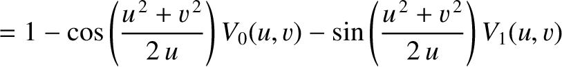
Likewise, in the geometric shadow region,
Lommel functions (Born and Wolf 1980)
(See Exercise 22.)
Likewise, in the geometric shadow region,  , the integrals can be expended in term of the convergent
 Lommel functions (Born and Wolf 1980)
(See Exercise 22.)
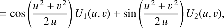
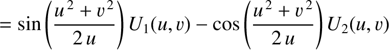
It follows (with the aid of some trigonometric identities) that
when , and
when .
Lommel functions (Born and Wolf 1980)
(See Exercise 22.)
It follows (with the aid of some trigonometric identities) that
when , and
when .
Figure 10.20:
Far/near-field diffraction pattern of a circular aperture. The left and right panels correspond to  and
and  , respectively. The thick black line indicates the physical extent of the aperture.
|
|
Finally, making use of Equation (10.110), the previous four equations imply that the
illumination intensity on the projection screen can be written
![$\displaystyle \frac{{\cal I}(v)}{{\cal I}_0}= \left[V_0(u,v)-\cos\left(\frac{u^...
...,2}
+ \left[V_1(u,v)-\sin\left(\frac{u^{\,2}+v^{\,2}}{2\,u}\right)\right]^{\,2}$](img3711.png) |
(10.161) |
when , and
![$\displaystyle \frac{{\cal I}(v)}{{\cal I}_0}= \left[U_1^{\,2}(u,v)+U_2^{\,2}(u,v)\right]$](img3712.png) |
(10.162) |
when . Here,
 is the intensity of the light illuminating the aperture from behind.
Figure 10.20 shows a typical far-field (i.e.,
) and near-field (i.e., )
diffraction pattern of a circular aperture, as determined from the previous analysis. It can be seen that
the far-field diffraction pattern is similar in form to that predicted by the simplified Fourier analysis
of Section 10.9. On the other hand, the near-field diffraction pattern is quite different. In fact,
the near-field diffraction pattern is fairly similar in
form to the geometric image of the aperture, apart from the presence of fringes within the image.


![\includegraphics[width=1\textwidth]{Chapter10/fig10_20.eps}](img3710.png)