Neoclassical Transport
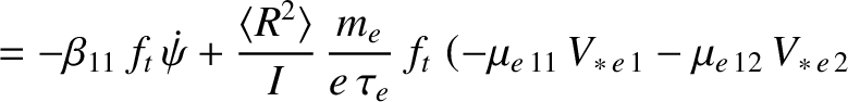
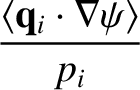
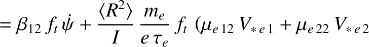
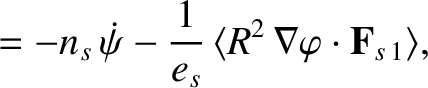
Taking the scalar product of Equations (2.163) and (2.164) with
 , and
flux-surface averaging, we obtain
where
and use has been made of Equations (2.130), (2.131), (2.155), (2.161), (2.162), (2.165), and (2.166).
Note that
, and
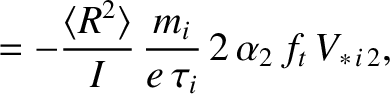
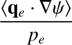
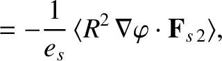
flux-surface averaging, we obtain
where
and use has been made of Equations (2.130), (2.131), (2.155), (2.161), (2.162), (2.165), and (2.166).
Note that
 and
and
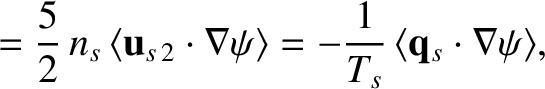
 are proportional to the species-
 particle and heat fluxes, respectively, across (i.e., perpendicular to) magnetic flux-surfaces. Note, further, that the cross-flux-surface components of the particle and
heat flow velocities are
particle and heat fluxes, respectively, across (i.e., perpendicular to) magnetic flux-surfaces. Note, further, that the cross-flux-surface components of the particle and
heat flow velocities are
 smaller than the in-flux-surface flow
velocities discussed in Section 2.11.
smaller than the in-flux-surface flow
velocities discussed in Section 2.11.
Now,
 |
(2.271) |
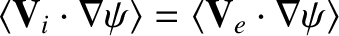
where use has been made of Equations (2.16) and (2.199). It follows that the cross-flux-surface
particle fluxes in tokamaks are automatically ambipolar, as a consequence of axisymmetry, quasi-neutrality, and collisional momentum conservation [44]. This result is of great significance because it implies that there is no preferred radial
electric field,
 , in a tokamak plasma, which means that the plasma can rotate freely
in the toroidal direction. [See Equations (2.228) and (2.231).] The situation is very different
in a non-axisymmetric magnetic confinement system, such as a stellarator, in which ambipolarity is
only attained at a certain value of the radial electric field. It follows that a stellarator plasma cannot
rotate freely in the toroidal direction [31].
, in a tokamak plasma, which means that the plasma can rotate freely
in the toroidal direction. [See Equations (2.228) and (2.231).] The situation is very different
in a non-axisymmetric magnetic confinement system, such as a stellarator, in which ambipolarity is
only attained at a certain value of the radial electric field. It follows that a stellarator plasma cannot
rotate freely in the toroidal direction [31].
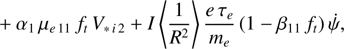
Equations (2.267) and (2.268) can be combined with Equations (2.186), (2.191), and (2.196) to give
where
Making use of Equations (2.193)–(2.195), (2.197), and (2.198), as well
as the large aspect-ratio approximation (2.230), we obtain
![$\displaystyle ({\mit\Gamma}_i)= -n_e\,(\skew{3}\dot{\psi}) +\frac{\langle R^2\r...
...llel\,e\,2}\\ [0.5ex] (15/2)\,(T_e/T_i)\,u_{\parallel\,i\,2}\end{array}\right),$](img1155.png) |
(2.276) |
 |
(2.277) |
 and
and
 . According to the previous
two equations, the large parallel particle and heat flows present in a low-collisionality plasma (see Sections 2.18 and 2.19) give rise to a transport of particles and heat across magnetic flux-surfaces. This transport,
which is far larger than the cross-flux-surface transport predicted by the classical closure scheme (see Section 2.6),
is known as neoclassical transport [22,43].
. According to the previous
two equations, the large parallel particle and heat flows present in a low-collisionality plasma (see Sections 2.18 and 2.19) give rise to a transport of particles and heat across magnetic flux-surfaces. This transport,
which is far larger than the cross-flux-surface transport predicted by the classical closure scheme (see Section 2.6),
is known as neoclassical transport [22,43].
Now, according to Equations (2.130), (2.131), (2.165), (2.166), (2.181), (2.221), (2.222), (2.243)–(2.250), (2.257), and (2.258),
It follows that
where use has been made of Equations (2.269) and (2.270). Note that we have also made use of the large aspect-ratio approximation that
 . Furthermore, we have neglected a
term that is
. Furthermore, we have neglected a
term that is
![${\cal O}[(m_e/m_i)^{1/2}]$](img1174.png) smaller than the leading-order term in Equation (2.282).
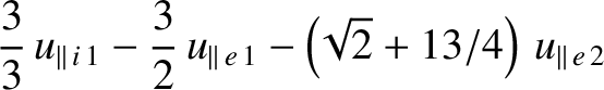
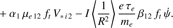
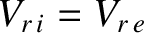
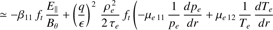
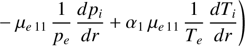
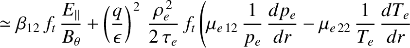
In the circular magnetic flux-surface limit, the previous three expressions reduce to [52]
and
smaller than the leading-order term in Equation (2.282).
In the circular magnetic flux-surface limit, the previous three expressions reduce to [52]
and
 |
(2.285) |
and
where use has been made of Equations (2.202), (2.209)–(2.211), (2.243), and (2.244).
The first term on the right-hand side of Equation (2.284) represents an inward flow of trapped particles driven by the inductive
parallel component of the electric field. This effect is know as the Ware pinch [51]. Consider the toroidal
component of the equation of motion of a particle of species :
 |
(2.287) |
(Note that  .) For a passing particle,
 is balanced by
 . In other words,
the toroidal electric field causes the toroidal velocity of the particle to continuously increase or decrease. This increase or decrease is
ultimately limited by collisions and parallel viscosity. [See Equation (2.175).] The net result is that
passing particles of both species carry a net toroidal current that is driven by the inductive electric field. For a trapped particle, on the other hand, the integral between bounces of the
left-hand side of the previous equation is zero. Thus, we obtain
. In other words,
the toroidal electric field causes the toroidal velocity of the particle to continuously increase or decrease. This increase or decrease is
ultimately limited by collisions and parallel viscosity. [See Equation (2.175).] The net result is that
passing particles of both species carry a net toroidal current that is driven by the inductive electric field. For a trapped particle, on the other hand, the integral between bounces of the
left-hand side of the previous equation is zero. Thus, we obtain
 |
(2.288) |
It follows that the time-averaged radial velocity of a trapped particle is
 |
(2.289) |
independent of the particle's mass or charge.
Hence, given that the trapped particle fraction is
 , we expect both plasma species to
exhibit a mean radial
flow of the form
, we expect both plasma species to
exhibit a mean radial
flow of the form
 |
(2.290) |
The Ware pinch does indeed have this form (when we take into account the fact that
 in a
large aspect-ratio tokamak).
It is clear from Equation (2.286) that the inward flow of trapped electrons is associated with an outward
electron heat flux.
in a
large aspect-ratio tokamak).
It is clear from Equation (2.286) that the inward flow of trapped electrons is associated with an outward
electron heat flux.
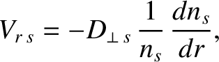
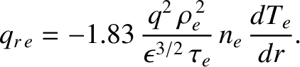
The remaining terms in Equations (2.284)–(2.286) are all diffusive in nature. According to Fick's
law [16], we expect the diffusive component of the species- radial velocity to take the form
 |
(2.291) |
where
 is the perpendicular (i.e., cross-flux-surface) particle diffusivity. If we ignore the Ware pinch and temperature gradient terms in Equation (2.284), and make the simplifying assumption that
  , then we
obtain
, then we
obtain
 |
(2.292) |
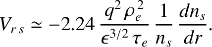
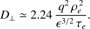
This leads to the following estimate for the perpendicular particle diffusivity (which is the same for
ions and electrons)
 |
(2.293) |
The previous equation can also be written
 |
(2.294) |
where use has been made of Equations (2.102) and (2.202).
The previous formula can be interpreted as follows. The collisions that scatter electrons out of their trapped orbits
displace the electrons across magnetic flux-surfaces a random distance that is of order the banana width,
 .
Such collisions take place at the frequency
.
Such collisions take place at the frequency
 . [See Equation (2.94).] Hence, the trapped
electrons have a diffusivity of
. [See Equation (2.94).] Hence, the trapped
electrons have a diffusivity of
 [41]. However, trapped electrons only make
up a fraction
[41]. However, trapped electrons only make
up a fraction  of the total number of electrons, so the overall electron diffusivity is
 [22,32,52].
Note that the ion diffusivity is limited to be the same as the electron diffusivity by the constraint that the
cross-flux-surface particle fluxes be ambipolar.
[22,32,52].
Note that the ion diffusivity is limited to be the same as the electron diffusivity by the constraint that the
cross-flux-surface particle fluxes be ambipolar.
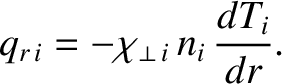
According to Fick's law [16], we expect the diffusive component of the ion heat flux to
take the form
 |
(2.295) |
We can see that Equation (2.285) does indeed take this form. Our estimate for the perpendicular ion energy diffusivity is thus
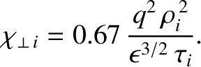 |
(2.296) |
The previous expression can also be written
 |
(2.297) |
We interpret the previous formula as saying that the neoclassical perpendicular ion energy diffusivity corresponds to the random-walk motions of
trapped ions with step-frequency
 and step-length
 [22,32,52].
Note that the neoclassical diffusivity specified in the previous equation is much larger, by a factor
[22,32,52].
Note that the neoclassical diffusivity specified in the previous equation is much larger, by a factor
 ,
that that predicted by the classical closure scheme. (See Section 2.6.)
,
that that predicted by the classical closure scheme. (See Section 2.6.)
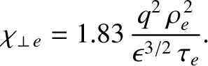
According to Fick's law [16], we expect the diffusive component of the electron heat flux to
take the form
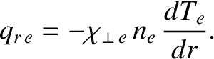 |
(2.298) |
If we neglect the Ware pinch, density gradient, and ion temperature gradient terms in Equation (2.286) then
we get
 |
(2.299) |
Hence, our estimate for the electron energy diffusivity becomes
 |
(2.300) |
The previous expression can also be written
 |
(2.301) |
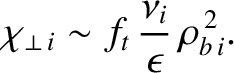
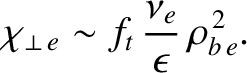
We interpret the previous formula as saying that the neoclassical perpendicular electron energy diffusivity corresponds to the random-walk motions of
trapped electrons with step-frequency
and step-length
[22,32,52].
As before, the neoclassical diffusivity specified in the previous equation is much larger, by a factor
,
that that predicted by the classical closure scheme. (See Section 2.6.)
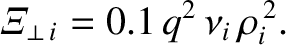
It turns out the the neoclassical cross-flux-surface momentum diffusivities only exceeds the classical
momentum diffusivities by a factor  . For example [52],
 |
(2.302) |
Table: 2.5
Neoclassical diffusivities in a low-field and a high-field tokamak reactor. Here,  is the toroidal
magnetic field-strength,
is the toroidal
magnetic field-strength,  the perpendicular particle diffusivity,
 the perpendicular electron energy diffusivity,
 the perpendicular ion energy diffusivity,
and
the perpendicular ion energy diffusivity,
and
 the perpendicular ion momentum diffusivity.
| |
Low-Field |
High-Field |
 |
5.0 |
12.0 |
 |
 |
|
 |
 |
|
 |
 |
|
 |
 |
|
|
Table 2.5 shows estimates for the neoclassical cross-flux-surface particle, heat, and momentum diffusivities in a tokamak
fusion reactor. Note that, although the diffusivities are much larger than the classical
cross-flux-surface diffusivities shown in Table 2.3, they are still all
much smaller than the experimentally observed cross-flux-surface diffusivities, which are
 and
and
 [52].
[52].

![$\displaystyle = \left(\begin{array}{c}
{\mit\Gamma}_{s\,1}\\ [0.5ex]
{\mit\Gamma}_{s\,2}
\end{array}\right),$](img1152.png)

![$\displaystyle = \left(\begin{array}{c}
\skew{3}\dot{\psi}\\ [0.5ex]
0
\end{array}\right).$](img1154.png)


![$\displaystyle = -n_e\,(\skew{3}\dot{\psi})
+ \frac{\langle R^2\rangle}{I}\,\fra...
...au_{ee}}
\left\{[E_{ii}]\,(u_{\varphi\,i})- [E_{ie}]\,(u_{\varphi\,e})\right\},$](img1148.png)

![$\displaystyle = -n_e\,(\skew{3}\dot{\psi})
-\frac{\langle R^2\rangle}{I}\,\frac...
...au_{ee}}
\left\{[F_{ee}]\,(u_{\varphi\,e})- [F_{ei}]\,(u_{\varphi\,i})\right\},$](img1150.png)

![$\displaystyle \left.\phantom{====}+ 0.19\,\frac{1}{T_e}\,\frac{dT_i}{dr}\right],$](img1179.png)

![$\displaystyle \left.\phantom{====}- 0.27\,\frac{1}{T_e}\,\frac{dT_i}{dr}\right],$](img1185.png)