Next: Lowest-Order Flows Up: Plasma Fluid Theory Previous: Drift and Transport Orderings Contents
 ,
,  ,
,  be a set of right-handed cylindrical coordinates whose symmetry axis corresponds to that of the
plasma equilibrium.
On the other hand, let
be a set of right-handed cylindrical coordinates whose symmetry axis corresponds to that of the
plasma equilibrium.
On the other hand, let  ,
,  , be a set of right-handed flux coordinates such that
  labels the equilibrium magnetic flux-surfaces, and increases by
 for every poloidal circuit of a given flux-surface. We can assume that
 without loss of generality. (Note that is a generalization of the poloidal angle introduced in Section 2.7 that does not assume that the flux-surfaces have circular cross-sections.) As before, we shall set
  on the outboard midplane. Note that
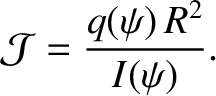
 . The Jacobean of our flux-coordinate
system is defined
. The Jacobean of our flux-coordinate
system is defined
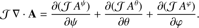
Now, a general vector field,  , can be written
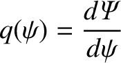
The axisymmetric equilibrium magnetic field of a tokamak can be expressed in the following manifestly divergence-free manner:
where . It follows that
 |
 |
(2.125) |
 |
 |
(2.126) |
 |
 |
(2.127) |
It is convenient to specialize to a coordinate system in which
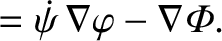
It follows thatThe equilibrium electric field is written
Here, , and
, and
 . Note that the previous equation automatically satisfies
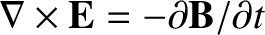 .
.
Finally, we expect the plasma equilibrium to be characterized by number density, temperature, and pressure profiles that
are flux-surface functions [18]. In other words,
 ,
,
 , and
, and
 . (See
Section 2.25.)
. (See
Section 2.25.)