Asymptotic Matching

The asymptotic matching relations (11.90) and (11.91) can be re-expressed in the forms (see Section 8.10),

$${\rm Re}\!\left(\frac{{\mit\Delta}\hat{\mit\Psi}_s}{\hat{\mit\Psi}_s}\right) =\frac{4\,\epsilon_\beta\,\epsilon_c}{\hat{w}}\int_{-1}^\infty\langle {\cal J}^{(c)}\,\cos\zeta\rangle\,d{\mit\Omega},$$ (11.140)

$${\rm Im}\!\left(\frac{{\mit\Delta}\hat{\mit\Psi}_s}{\hat{\mit\Psi}_s}\right) =-\frac{4\,\epsilon_\beta\,\epsilon_c}{\hat{w}}\int_{-1}^\infty\l... ...-1}^\infty\, \langle X\,\{{\cal J}^{(s)},{\mit\Omega}\}\rangle \,d{\mit\Omega}.$$ (11.141)

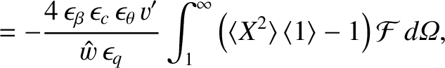
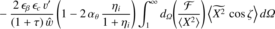
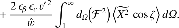
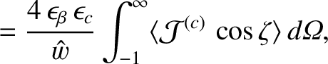
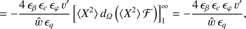
Equations (11.123), (11.136), and (11.141) yield

$${\rm Im}\!\left(\frac{{\mit\Delta}\hat{\mit\Psi}_s}{\hat{\mit\Psi... ...e X^{\,2}\rangle-\vert X\vert\right){\cal F}\right]\right\rangle d{\mit\Omega}.$$ (11.142)

Employing the easily proved identity $\langle X^{\,2}\,\partial_{\mit\Omega} G\rangle \equiv \partial_{\mit\Omega}\langle X^{\,2}\,G\rangle - \langle G\rangle$, we obtain

$${\rm Im}\!\left(\frac{{\mit\Delta}\hat{\mit\Psi}_s}{\hat{\mit\Psi}_s}\right) =\frac{4\,\epsilon_\beta\,\epsilon_c\,\epsilon_\theta\,v'}{\hat{w... ...nfty \left(\langle X^2\rangle\,\langle 1\rangle-1\right){\cal F}\,d{\mit\Omega}$$

$$= - \frac{4\,\epsilon_\beta\,\epsilon_c\,\epsilon_\theta\,v'}{\ha... ...fty \left(\langle X^2\rangle\,\langle 1\rangle-1\right){\cal F}\,d{\mit\Omega},$$ (11.143)

where use has been made of Equations (11.138), (11.139), as well as the fact that $\langle X^{\,2}\rangle^2-\langle\vert X\vert^{\,3}\rangle\sim {\mit\Omega}^{\,-1}$ as ${\mit\Omega}\rightarrow\infty$. However, according to Equation (11.137),

$${\rm Im}\!\left(\frac{{\mit\Delta}\hat{\mit\Psi}_s}{\hat{\mit\Psi}_s}\right) = -\frac{4\,\epsilon_\beta\,\epsilon_c\,\epsilon_\varphi\,v'}{\ha... ...frac{4\,\epsilon_\beta\,\epsilon_c\,\epsilon_\varphi\,v'}{\hat{w}\,\epsilon_q},$$ (11.144)

where use has been made of Equations (11.138) and (11.139). The previous equation yields

$$\left[r\,\frac{d\omega_E}{dr}\right]_{r_{s-}}^{r_{s+}}=\left(\fra... ...) {\rm Im}\!\left(\frac{{\mit\Delta}\hat{\mit\Psi}_s}{\hat{\mit\Psi}_s}\right),$$ (11.145)

where use has been made of Equations (8.23), (8.25), (8.27), and (8.46), and (8.103). Here, $\tau _H$ is the hydromagnetic time [see Equation (5.43)], and $\tau _\varphi$ is the toroidal momentum confinement time [see Equation (5.50)]. Equation (11.145) can also be obtained by integrating Equation (3.165) across the rational surface, making use of Equation (3.140), as well as the identification

$$\left[r\,\frac{d\omega_E}{dr}\right]_{r_{s-}}^{r_{s+}} = -n\left[r\,\frac{\partial{\mit\Delta\Omega}_z}{\partial r}\right]_{r_{s-}}^{r_{s+}}.$$ (11.146)

If we compare Equation (11.145) with Equation (8.102) then we can see that the discontinuity in the MHD fluid velocity gradient that develops at the rational surface is a factor $(\epsilon_s/q_s)^2$ smaller in our neoclassical drift-MHD model than the corresponding discontinuity in our non-neoclassical drift-MHD model. The reason for this reduction is that the strong poloidal flow-damping present in the former model prevents the poloidal plasma rotation profile from being modified by the localized electromagnetic torque produced at the rational surface. Instead, only the toroidal plasma rotation profile is modified by the electromagnetic torque [4,18].

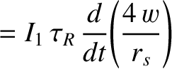
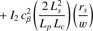
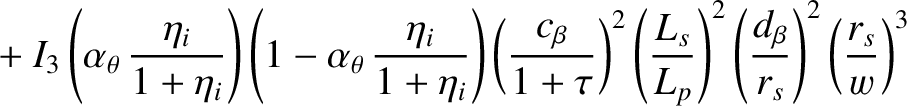
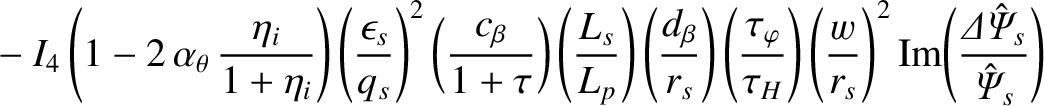
It follows from Equations (11.113), (11.127), (11.130), (11.136), and (11.140) that

$${\rm Re}\!\left(\frac{{\mit\Delta}\hat{\mit\Psi}_s}{\hat{\mit\Psi}_s}\right) = \frac{4}{\epsilon_R\,\hat{w}}\,\frac{d(\ln \hat{w}^2)}{dT}\int_... ...{\langle \cos\zeta\rangle}{\langle 1\rangle\,\langle X^2\rangle}\,d{\mit\Omega}$$

$$\phantom{=}-\frac{4\,\epsilon_\beta\,\epsilon_c\,\zeta_g}{\hat{w}... ... \widetilde{\vert X\vert}\,\cos\zeta\rangle}{\langle X^2\rangle}\,d{\mit\Omega}$$

$$\phantom{=}- \frac{2\,\epsilon_\beta\,\epsilon_c}{(1+\tau)^2\,\ha... ...gle^2}\right)\left\langle \widetilde{X^2}\,\cos\zeta\right\rangle d{\mit\Omega}$$

$$\phantom{=}-\frac{2\,\epsilon_\beta\,\epsilon_c\,v'}{(1+\tau)\,\h... ...angle}\right)\left\langle \widetilde{X^2}\,\cos\zeta\right\rangle d{\mit\Omega}$$

$$\phantom{=}+\frac{2\,\epsilon_\beta\,\epsilon_c\,v'^{\,2}}{\hat{w... ... F}^2\right)\left\langle \widetilde{X^2}\,\cos\zeta\right\rangle d{\mit\Omega}.$$ (11.147)

Here,

$${\cal H}({\mit\Omega})=\left\{ \begin{array}{llr} 0&&-1\leq {... ...\Omega}\leq 1\\ [0.5ex] 1&~~&{\mit\Omega}>1 \end{array}\right.,$$ (11.148)

and use has been made of the fact that ${\cal F}({\mit\Omega})$ is continuous across the separatrix. The previous equation can be combined with Equations (8.10), (8.23)–(8.27), (8.103), and (11.77), (11.79), and (11.144) to give [2,3,7,14,15,20,21,23]

$${\rm Re}\!\left(\frac{{\mit\Delta}\hat{\mit\Psi}_s}{\hat{\mit\Psi}_s}\right) = I_1\,\tau_R\,\frac{d}{dt}\!\left(\frac{4\,w}{r_s}\right)$$

$$\phantom{=}-I_2\left[\beta_{11}\left(1-\alpha_1\,\frac{1}{1+\tau}... ...psilon_s}\right)c_\beta^2\left(\frac{L_s}{L_p}\right)\left(\frac{r_s}{w}\right)$$

$$\phantom{=}+I_2\,c_\beta^2\left(\frac{2\,L_s^2}{L_p\,L_c}\right)\left(\frac{r_s}{w}\right)$$

$$\phantom{=}+I_3\left(\alpha_\theta\,\frac{\eta_i}{1+\eta_i}\right... ...{L_p}\right)^2\left(\frac{d_{\beta}}{r_s}\right)^2 \left(\frac{r_s}{w}\right)^3$$

$$\phantom{=}- I_4\left(1-2\,\alpha_\theta\,\frac{\eta_i}{1+\eta_i}... ...)^2{\rm Im}\!\left(\frac{{\mit\Delta}\hat{\mit\Psi}_s}{\hat{\mit\Psi}_s}\right)$$

$$\phantom{=}- I_5 \left(\frac{\epsilon_s}{q_s}\right)^4\left(\frac... ...left(\frac{{\mit\Delta}\hat{\mit\Psi}_s}{\hat{\mit\Psi}_s}\right)\right]^{\,2}.$$ (11.149)

where

$$I_1 = 2\int_{-1}^\infty \frac{\langle \cos\zeta\rangle^2}{\langle 1\rangle}\,d{\mit\Omega},$$ (11.150)

$$I_2 = 2\int_1^{\infty}\left(\frac{\langle \vert X\vert^3\rangle}{\langle X^2\rangle}-\frac{1}{\langle 1\rangle}\right)d{\mit\Omega},$$ (11.151)

$$I_3 = \int_{1-}^\infty d_{\mit\Omega}\!\left(\frac{{\cal H}}{\langle ... ...X^4\rangle - \frac{\langle X^2\rangle^2}{\langle 1\rangle}\right)d{\mit\Omega},$$ (11.152)

$$I_4 = \frac{1}{4}\int_1^\infty d_{\mit\Omega}\!\left(\frac{{\cal F}}{... ...X^4\rangle - \frac{\langle X^2\rangle^2}{\langle 1\rangle}\right)d{\mit\Omega},$$ (11.153)

$$I_5 = \frac{1}{16}\int_1^\infty d_{\mit\Omega}\!\left({\cal F}^{\,2}\... ...X^4\rangle - \frac{\langle X^2\rangle^2}{\langle 1\rangle}\right)d{\mit\Omega}.$$ (11.154)