Higher-Order Solution

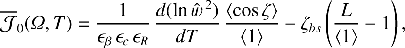
Our zeroth-order solution is characterized by three undetermined flux-surface functions: $\overline{{\cal J}}_0({\mit\Omega},T)$, $L({\mit\Omega},T)$, and $F({\mit\Omega},T)$. In order to determine the forms of these functions, we need to expand our model to higher order. (See Section 8.8.)

Expanding Equation (11.68) to third order in $\epsilon$, we obtain we obtain

$$\frac{d(\ln \hat{w}^{\,2})}{dT}\,\cos\zeta = \{F_e, {\mit\Omega}\... ...eta_{bs}\,\epsilon_\beta\,\epsilon_c\,\epsilon_R\left(\vert X\vert\,L-1\right),$$ (11.124)

where

$$F_e({\mit\Omega},\zeta,T)= \epsilon^2\,({\mit\Phi}_2+\epsilon\,{\... ...\cal N}_3) - \epsilon^2\,\varsigma\,Y_e\,({\mit\Psi}_2+\epsilon\,{\mit\Psi}_3),$$ (11.125)

and use has been made of Equations  (8.75), (11.95)–(11.99), (11.103), (11.104), (11.107), and (11.108). The flux-surface average of Equation (11.124) yields

$$\overline{\cal J}_0({\mit\Omega},T)= \frac{1}{\epsilon_\beta\,\ep... ...rangle}{\langle 1\rangle}-\zeta_{bs}\left(\frac{L}{\langle 1\rangle} -1\right),$$ (11.126)

where use has been made of Equations (8.68), (8.70), and (11.114), and (11.116). Note that $\langle{\cal J}_0^{(s)}\rangle=0$, by symmetry. Hence,

$${\cal J}_0^{(c)}({\mit\Omega},\zeta,T) = \frac{1}{\epsilon_\beta\,\epsilon_c\,\epsilon_R}\,\frac{d(\ln\h... ...left(\frac{L}{\langle 1\rangle} -1\right) -\zeta_g\,L\,\widetilde{\vert X\vert}$$

$$\phantom{=}+\frac{1}{2}\,\partial_{\mit\Omega}\!\left[M\left(M+ \frac{L}{1+\tau}\right)\right]\,\widetilde{X^{\,2}},$$ (11.127)

where use has been made of Equation (11.116).

Expanding Equation (11.69) to first order in $\epsilon$, we obtain

$$0= \epsilon\,\{{\cal V}_1, {\mit\Omega}\} + \epsilon^2\,\epsilon_... ...\Omega}\right\}+ \epsilon_\perp\,\varsigma\,(X^2\,\partial_{\mit\Omega} L + L),$$ (11.128)

where use has been made of Equations (11.95)–(11.99), (11.101), (11.103), and (11.104). The flux-surface average of the previous equation yields

$$\partial_{\mit\Omega}\!\left(\langle X^{\,2}\rangle\,L\right) = 0.$$ (11.129)

We can solve the previous equation, subject to the boundary condition (11.105), to give

$$L({\mit\Omega},T)= L({\mit\Omega})=\left\{ \begin{array}{llr}... ...5ex] 1/\langle X^2\rangle&~~&{\mit\Omega}>1 \end{array}\right..$$ (11.130)

Here, we have taken into account the previously mentioned fact that $L=0$ within the island separatrix. Note that $L({\mit\Omega})$ is discontinuous across the island separatrix, which implies that the pressure gradient is also discontinuous across the separatrix. As discussed in Section 8.9, we expect this discontinuity to be resolved in a layer of characteristic thickness $4\,w_d$ on the separatrix [see Equation (8.84) and Table 8.1].

Expanding Equation (11.71) to second order in $\epsilon$, we obtain we obtain

$$=\epsilon\left\{-\epsilon_c\,\varsigma\,M\,{\cal V}_1-\epsilon\,\... ...ga}\right\} -\epsilon_c\,\epsilon_\theta\,({\cal V}_{(0)}-\xi\,\vert X\vert\,F)$$ 0

$$\phantom{=}+ \epsilon_c\,\epsilon_\varphi\left(X^2\,\partial_{\mit\Omega}^2 {\cal V}_{(0)} + \partial_{\mit\Omega}{\cal V}_{(0)}\right),$$ (11.131)

where use has been made of Equations (11.95)–(11.99), (11.101), (11.103), (11.104), (11.107), (11.108), (11.111), and (11.113). The flux-surface average of the previous equation yields

$$\epsilon_\varphi\,\partial_{\mit\Omega}\!\left(\langle X^{\,2}\ra... ...}\right) =\epsilon_\theta\left(\langle 1\rangle\, {\cal V}_{(0)}-\xi\,F\right).$$ (11.132)

According to Equation (11.121), recalling that $F({\mit\Omega}\leq 1,T)=0$, we get

$$0 =\epsilon_\theta\,\langle 1\rangle \,c_0(T)$$ (11.133)

inside the separatrix, which implies that $c_0(T)=0$. Hence, given that we have already concluded that $c_1(T)= 0$, Equations (11.121) and (11.122) yield

$${\cal V}_{(0)}({\mit\Omega},T)= \xi\,\langle X^{\,2}\rangle\,F({\mit\Omega}, T).$$ (11.134)

The previous equation can be combined with Equation (11.132) to produce

$$\epsilon_\varphi\,\partial_{\mit\Omega}\!\left[\langle X^{\,2}\ra... ...ht] = \epsilon_\theta\left(\langle X^{\,2}\rangle\,\langle 1\rangle -1\right)F.$$ (11.135)

Now, it is apparent from the previous equation that there is no discontinuity in $F$ across the separatrix. Thus, given that $F({\mit\Omega}\leq 1,T)=0$, it follows that $F(1_+,T)=0$. It is also clear from Equations (11.105), (11.109), and (11.113) that $F({\mit\Omega}\rightarrow\infty, T)= v'(T)$. Thus, we can write

$$F({\mit\Omega},T)=v'(T)\left\{ \begin{array}{llr} 0&&-1\leq {... ...x] {\cal F}({\mit\Omega})&~~&{\mit\Omega}>1 \end{array}\right.,$$ (11.136)

where

$$\epsilon_\varphi\,d_{\mit\Omega}\!\left[\langle X^{\,2}\rangle\,d... ...epsilon_\theta\left(\langle X^{\,2}\rangle\,\langle 1\rangle -1\right){\cal F},$$ (11.137)

and

$${\cal F}(1) =0,$$ (11.138)

$${\cal F}({\mit\Omega}\rightarrow\infty) = 1.$$ (11.139)

Here, $d_{\mit\Omega}\equiv d/d{\mit\Omega}$.