Next: Improved Torque Balance Model Up: Rotation Braking in Tokamak Previous: Rotation Braking by a Contents
 ), the critical wall thickness above which the thin-wall
approximation fails is
), the critical wall thickness above which the thin-wall
approximation fails is
 m. For the case of a
high-field reactor, the critical wall thickness is
m. For the case of a
high-field reactor, the critical wall thickness is
 m.
It follows that the thin-wall approximation holds for resistive walls (i.e.,
m.
It follows that the thin-wall approximation holds for resistive walls (i.e.,
 ),
but not for highly conducting walls (i.e.,
),
but not for highly conducting walls (i.e.,
 ), because the latter type of wall would have to be impossibly thin.
A second deficiency in our previous calculation is that it neglects plasma inertia. This neglect is reasonable when the magnetic island chain is rotating steadily, but not when the chain's rotation frequency collapses, because such a collapse is associated with a rapid deceleration of the chain, and a consequent rapid deceleration of the plasma in the vicinity of the resonant surface.
A third deficiency in our previous calculation is that it assumes that the eddy current excited in the
wall has a simple
 time dependence, where
  is the instantaneous rotation frequency
of the island chain. This assumption is reasonable when the island chain is rotating steadily, but not
when its rotation frequency collapses, in which case we expect the rapid deceleration of the
chain to excite a transient eddy current in the wall [4].
is the instantaneous rotation frequency
of the island chain. This assumption is reasonable when the island chain is rotating steadily, but not
when its rotation frequency collapses, in which case we expect the rapid deceleration of the
chain to excite a transient eddy current in the wall [4].
The aim of this section is to generalize the analysis of the previous section in order to take into account thick walls,
plasma inertia, and a transient component of the wall eddy current.
Note that, by a “thick” wall, we mean one in which the skin-depth in the wall material is less than the wall's radial thickness. It is still reasonable to assume that the wall's thickness,  , is much less than its minor radius,
  .
.
Suppose that the wall extends from  to
to
 , where
 . Here,
  is
a conventional cylindrical coordinate.
Let
is
a conventional cylindrical coordinate.
Let
 be the perturbed magnetic flux within the wall [see Equation (3.20)]. Here,
  is the equilibrium toroidal magnetic field-strength. Ohm's
law inside the wall yields [see Equation (3.101)]
is the equilibrium toroidal magnetic field-strength. Ohm's
law inside the wall yields [see Equation (3.101)]
 is the electrical resistivity of the wall material.
The previous equation must be solved subject to the boundary conditions
is the electrical resistivity of the wall material.
The previous equation must be solved subject to the boundary conditions
 |
 |
(10.32) |
 |
 |
(10.33) |
 to be the normalized helical magnetic flux that penetrates the inner (in ) boundary of the wall. The second boundary condition follows
because, in the vacuum region outside the
wall, a well-behaved solution of the cylindrical tearing mode equation, (3.60), varies as
to be the normalized helical magnetic flux that penetrates the inner (in ) boundary of the wall. The second boundary condition follows
because, in the vacuum region outside the
wall, a well-behaved solution of the cylindrical tearing mode equation, (3.60), varies as  .
.
Let
Equations (10.31)–(10.33) yield whereLet us, first, search for a solution of
 |
 |
(10.42) |
 |
 |
(10.43) |
 |
 |
(10.44) |
Let us write
where Expression (10.50) automatically satisfies the boundary conditions (10.37) and (10.38). It is clear, by analogy with Equation (10.49), that if the inequality (10.47) is satisfied then the boundary condition (10.52) effectively reduces to Let us write where |
(10.55) |
 |
(10.57) |
 , and integrating from
  to
to  , we obtain
[4]
where
, we obtain
[4]
where
 |
(10.59) |
 |
 |
(10.60) |
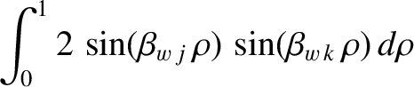
![$\displaystyle \int_0^1\left\{
\frac{(\rho-1)\,\sinh[\alpha_w\,(\rho-1)]}{\cosh\...
...ho-1)]\,\sinh\alpha_w}{\cosh^2\alpha_w}\right\}
\sin(\beta_{w\,j}\,\rho)\,d\rho$](img3177.png) |
 |
|
 |
 |
(10.61) |
Equation (3.83) generalizes to give
![$\displaystyle {\mit\Delta\hat{\Psi}}_w =
\left[r\,\frac{\partial \delta\hat{\ps...
...si}_w}{\zeta_w}\left[\frac{\partial F}{\partial \rho}\right]_{\rho=0}^{\rho=1},$](img3181.png) |
(10.62) |
 is a measure of the normalized net eddy current induced in the wall.
It follows from Equations (10.48), (10.46), (10.50), and (10.54) that [4]
where
Clearly, Equation (10.63) specifies the relation between the net eddy current induced in the wall and the helical magnetic flux that penetrates the inner boundary of the wall.
is a measure of the normalized net eddy current induced in the wall.
It follows from Equations (10.48), (10.46), (10.50), and (10.54) that [4]
where
Clearly, Equation (10.63) specifies the relation between the net eddy current induced in the wall and the helical magnetic flux that penetrates the inner boundary of the wall.
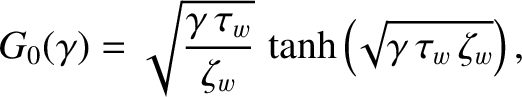
The first term on the right-hand side of the Equation (10.64),
specifies the net eddy current induced in the wall by a steadily rotating island chain. In the thin-wall limit [see Equations (3.104), (10.39), (10.41), and (10.47)] [4], |
(10.66) |
 |
(10.67) |
 |
(10.68) |
 |
(10.69) |
The second term on the right-hand side of Equation (10.64),
 |
(10.70) |
 ) changes in time.
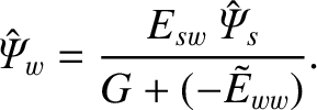
Equation (3.188) (with
 , because there is no error-field) and Equation (10.63) yield
 |
(10.72) |
 is the instantaneous island rotation frequency, Equations (10.39) and
(10.71) imply that
Here, we have made use of the fact that
is the instantaneous island rotation frequency, Equations (10.39) and
(10.71) imply that
Here, we have made use of the fact that
 [see Equation (8.1)].
Equations (3.187) and (10.71) give
[see Equation (8.1)].
Equations (3.187) and (10.71) give
![$\displaystyle \frac{{\mit\Delta\hat{\Psi}}_s}{\hat{\mit\Psi}_s}=
{\mit\Delta}_{...
...lta}_{pw}(0)\right]\left[\frac{(-\tilde{E}_{ww})}{G+ (-\tilde{E}_{ww})}\right],$](img3196.png) |
(10.74) |
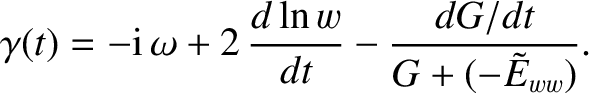
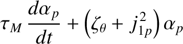
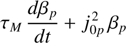
Equations (8.108), (10.75), and (10.76) yield the following modified Rutherford island width evolution equation, which is a generalization of Equation (10.9):
All of the parameters appearing in this equation are defined in the previous section.As in the previous section, the instantaneous island rotation frequency can be written [see Equation (10.10)]
 |
(10.80) |
 and
and  is specified by
where all of the parameters appearing in the previous two equations are defined in the previous section,
except for
is specified by
where all of the parameters appearing in the previous two equations are defined in the previous section,
except for
 |
 |
(10.83) |
 |
 |
(10.84) |
 |
![$\displaystyle = \left[\frac{J_1(j_{1p}\,r_s/a)}{J_2(j_{1p})}\right]^2,$](img3215.png) |
(10.85) |
 |
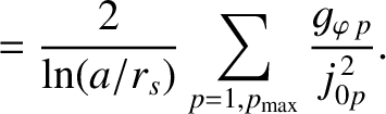
![$\displaystyle = \left[\frac{J_0(j_{0p}\,r_s/a)}{J_1(j_{0p})}\right]^2.$](img3217.png) |
(10.86) |
 and
and  are standard Bessel functions, and
  denotes the
  th
zero of the
th
zero of the  Bessel function [1]. Note that the terms involving
  in Equations (10.81)
and (10.82) represent plasma inertia.
in Equations (10.81)
and (10.82) represent plasma inertia.
Let
 ,
,
 , and
, and
 . Thus,
  is the width of the magnetic island chain relative to its saturated width when the wall is perfectly conducting,
  is the island
rotation frequency relative to the magnitude of its value when there is no interaction with the wall, and
is the island
rotation frequency relative to the magnitude of its value when there is no interaction with the wall, and  is time
normalized to the typical time required for the island chain complete a full rotation.
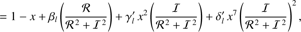
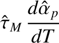
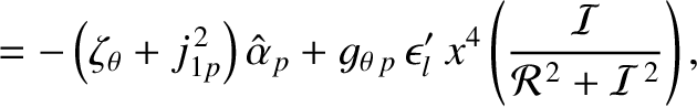
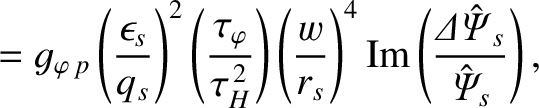
Equations (10.73) and (10.75)–(10.82) can be converted into the following closed set of normalized equations that govern the time evolution of
the island chain's rotation frequency:
is time
normalized to the typical time required for the island chain complete a full rotation.
Equations (10.73) and (10.75)–(10.82) can be converted into the following closed set of normalized equations that govern the time evolution of
the island chain's rotation frequency:
 |
 |
(10.88) |
 |
 |
(10.89) |
 |
 |
(10.90) |
 |
 |
(10.93) |
 is specified in Equation (10.20),
 is specified in Equation (10.84), and
Note that , ,
is specified in Equation (10.84), and
Note that , ,
 and
and
 are real quantities, whereas
 and
and  are complex.
The type of rotation braking calculation discussed in this section is far more computationally intensive than the type discussed in the previous section, because the former type involves the solution of a great many more differential equations than the latter. However, the new calculation is an improvement on the previous one because it allows us to determine the time scale on which rotating braking occurs. Our previous calculation is unable to achieve this goal because it neglects plasma inertia.
Let us investigate a specific example.
Consider a high-field tokamak fusion reactor (see Chapter 1) characterized by
 ,
,
 ,
,
 ,
,
 (where
  and
and  are the deuteron and triton masses, respectively),
 ,
,  ,
,
 ,
,
 ,
,
 . The wall parameters are
 (which is the electrical resistivity of stainless steel),
 , and
, and
 .
The plasma equilibrium is
assumed to be of the Wesson type (see Section 9.4), with
.
The plasma equilibrium is
assumed to be of the Wesson type (see Section 9.4), with  and
and  .
The poloidal and toroidal mode numbers of the tearing mode are
.
The poloidal and toroidal mode numbers of the tearing mode are  and
and  , respectively. It follows that
 . The perfect-wall saturated
island width is
. The perfect-wall saturated
island width is
 , the poloidal flow-damping time is
 s, the wall time-constant is
 , the momentum
confinement time is
, the momentum
confinement time is
 [see Equation (3.180)], and the typical type required for
the magnetic island to attain its final saturated width is
[see Equation (3.180)], and the typical type required for
the magnetic island to attain its final saturated width is
 . The normalized
parameters that characterize our model take the values
. The normalized
parameters that characterize our model take the values
 ,
,
 ,
,
 ,
,
 ,
,
 ,
,
 ,
,
 ,
,
 ,
,
 , and
, and
 . We conclude that the effective L/R time of the wall is
about
. We conclude that the effective L/R time of the wall is
about  times larger than the typical time required for the unperturbed magnetic island chain to complete a full rotation
(i.e.,
times larger than the typical time required for the unperturbed magnetic island chain to complete a full rotation
(i.e.,
 ),
the momentum confinement time is about
),
the momentum confinement time is about  times larger than the island rotation time (i.e.,
 ), and the island saturation time is
about
), and the island saturation time is
about
 times larger than the island rotation time (i.e.,
 ).
).
![\includegraphics[width=\textwidth]{Chapter10/Figure10_5.eps}](img3289.png)
|
It turns out that 100
poloidal and toroidal velocity harmonics are sufficient to describe the time evolution of the plasma poloidal and toroidal rotation profiles in a reasonably accurate manner. Consequently, we shall neglect all and variables
with
 in our calculation. In order to compensate for the truncation of the sum in
Equation (10.87), we shall replace this equation by
in our calculation. In order to compensate for the truncation of the sum in
Equation (10.87), we shall replace this equation by
 |
 |
(10.107) |
 |
 |
(10.108) |
 and
and
 .
.
For the transient wall harmonics, an examination of Equations (10.95) and (10.97) implies that, roughly speaking,
that all harmonics in the range
 , where
 , are important in the calculation. Hence,
given that
, are important in the calculation. Hence,
given that
 ,
we deduce from Equation (10.96) that
,
we deduce from Equation (10.96) that
 . This result merely implies that when the island chain
is rotating at its unperturbed rotation frequency the transient eddy current induced in the wall only penetrates radially into about the inner 7th part of the wall. Hence, we need to retain all transient wall harmonics up to of order
. This result merely implies that when the island chain
is rotating at its unperturbed rotation frequency the transient eddy current induced in the wall only penetrates radially into about the inner 7th part of the wall. Hence, we need to retain all transient wall harmonics up to of order  in order to resolve this relatively thin current distribution.
In the following, we shall keep all transient wall harmonics up to
in order to resolve this relatively thin current distribution.
In the following, we shall keep all transient wall harmonics up to  (i.e., we shall neglect
  variables with
 in our calculation), so as to ensure that all important transient wall harmonics are retained in the calculation.
It follows that the final set of coupled, first-order, ordinary differential equations that makes up our model consists of
243 real equations.
in our calculation), so as to ensure that all important transient wall harmonics are retained in the calculation.
It follows that the final set of coupled, first-order, ordinary differential equations that makes up our model consists of
243 real equations.
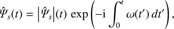
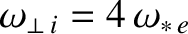
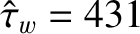
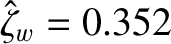
Figure 10.5 shows the numerical solution of our set of differential equations. The solution is qualitatively similar
to that obtained for a thin wall. (See Figure 10.2.) As before, it can be seen that as the normalized width, , of the island chain grows in time, the chain's normalized rotation frequency, , is gradually reduced, until
it has been reduced to about half of its original value, at which point there is a sudden collapse in the
rotation frequency to a very low value. The rotation collapse occurs when  , which corresponds to
 .
It is clear from the right-hand panel of Figure 10.5 that the
rotation collapse takes place over a time interval of about 100 normalized time units, which corresponds to about
15 ms. This timescale is
similar to the hybrid timescale
.
It is clear from the right-hand panel of Figure 10.5 that the
rotation collapse takes place over a time interval of about 100 normalized time units, which corresponds to about
15 ms. This timescale is
similar to the hybrid timescale
 ms.
Hence, it is plausible that the timescale for the rotation collapse is
determined by a combination of poloidal flow damping and perpendicular viscosity.
ms.
Hence, it is plausible that the timescale for the rotation collapse is
determined by a combination of poloidal flow damping and perpendicular viscosity.
![\includegraphics[width=\textwidth]{Chapter10/Figure10_6.eps}](img3309.png)
|
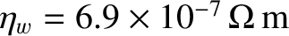
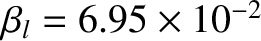
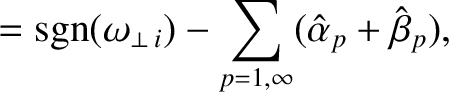
We can construct a torque balance diagnostic:
 |
(10.109) |
 is specified in Equation (10.12).
The
quantity
is specified in Equation (10.12).
The
quantity  takes the value zero when the plasma is in torque balance. In other words, when the
electromagnetic braking torque exerted at the rational surface is exactly balanced by the viscous
restoring torque. Obviously, plasma inertia plays no role in the rotation braking process when the plasma
is in torque balance. On the other hand, if is non-zero then the electromagnetic braking torque
is not balanced by the viscous restoring torque, which indicates that plasma inertia is playing a role in the
braking process. Figure 10.6 displays the time evolution of the torque balance diagnostic in the rotation braking simulation
shown in Figure 10.5. It can be seen that the plasma is in torque balance to a very good approximation
both before and after the rotation collapse. However, during the rotation collapse, the plasma is clearly not in
torque balance, indicating that plasma inertia plays an important role in the rotation collapse.
According to the right-hand panel of Figure 10.6, after torque balance breaks down during the rotation
collapse, it takes a time interval of order 4000 normalized time units, which corresponds to about
takes the value zero when the plasma is in torque balance. In other words, when the
electromagnetic braking torque exerted at the rational surface is exactly balanced by the viscous
restoring torque. Obviously, plasma inertia plays no role in the rotation braking process when the plasma
is in torque balance. On the other hand, if is non-zero then the electromagnetic braking torque
is not balanced by the viscous restoring torque, which indicates that plasma inertia is playing a role in the
braking process. Figure 10.6 displays the time evolution of the torque balance diagnostic in the rotation braking simulation
shown in Figure 10.5. It can be seen that the plasma is in torque balance to a very good approximation
both before and after the rotation collapse. However, during the rotation collapse, the plasma is clearly not in
torque balance, indicating that plasma inertia plays an important role in the rotation collapse.
According to the right-hand panel of Figure 10.6, after torque balance breaks down during the rotation
collapse, it takes a time interval of order 4000 normalized time units, which corresponds to about
 s, for torque balance to be
reestablished. This timescale is similar to the momentum confinement timescale,
s, for torque balance to be
reestablished. This timescale is similar to the momentum confinement timescale,
 s. Hence,
it is plausible that torque balance is reestablished by plasma viscosity.
s. Hence,
it is plausible that torque balance is reestablished by plasma viscosity.
![\includegraphics[width=\textwidth]{Chapter10/Figure10_7.eps}](img3318.png)
|
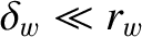
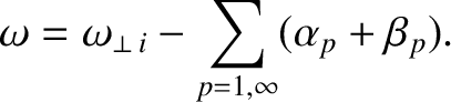
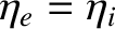
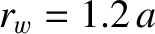
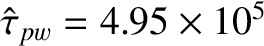
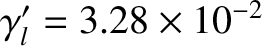
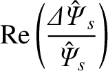
Figure 10.7 shows the time evolution of the quantities
in the rotation braking simulation shown in Figure 10.5. Now, the rotation braking process causes the normalized rotation frequency of the island chain,, to decrease from unity (assuming that
 ) to a value that is very much smaller than unity. In other
words,
) to a value that is very much smaller than unity. In other
words,
 . Hence, it is clear from Equations (10.106), (10.111),
and (10.112) that
. Hence, it is clear from Equations (10.106), (10.111),
and (10.112) that
 . Here,
 is the fraction of the decrease in the island rotation frequency that is due to a shift in the
poloidal ion fluid angular velocity at the rational surface, whereas
is the fraction of the decrease in the island rotation frequency that is due to a shift in the
poloidal ion fluid angular velocity at the rational surface, whereas
 is the fraction of the decrease that is
due to a shift in the toroidal ion fluid angular velocity at the rational surface. In fact, it is apparent from Figure 10.7 that about 53% of
the decrease in the rotation frequency is due to a poloidal velocity shift, the remaining 47% being due to
a toroidal velocity shift. It is also apparent from the figure's right-hand panel that the rotation collapse, which takes place on
a timescale of about 100 normalized time units [i.e.,
is the fraction of the decrease that is
due to a shift in the toroidal ion fluid angular velocity at the rational surface. In fact, it is apparent from Figure 10.7 that about 53% of
the decrease in the rotation frequency is due to a poloidal velocity shift, the remaining 47% being due to
a toroidal velocity shift. It is also apparent from the figure's right-hand panel that the rotation collapse, which takes place on
a timescale of about 100 normalized time units [i.e.,
 ], is due to a sudden shift in the poloidal angular velocity at the rational surface. In fact, this sudden shift is responsible for the loss of
torque balance during the rotation collapse. The corresponding shift in the toroidal angular velocity at the rational surface takes place
on a timescale of 4000 normalized time units (i.e.,
], is due to a sudden shift in the poloidal angular velocity at the rational surface. In fact, this sudden shift is responsible for the loss of
torque balance during the rotation collapse. The corresponding shift in the toroidal angular velocity at the rational surface takes place
on a timescale of 4000 normalized time units (i.e.,  ). Note that, after the sudden shift that is associated with rotation collapse, the poloidal velocity subsequently readjusts to its final value on the timescale.
![\includegraphics[width=\textwidth]{Chapter10/Figure10_8.eps}](img3329.png)
|
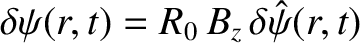
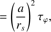
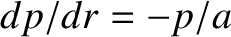
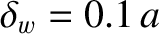
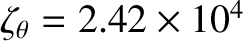
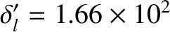
Figure 10.8 shows the time evolution of the transient wall harmonics in the rotation braking
simulation shown in Figure 10.5. It can be seen that the transient wall harmonics are
only important [i.e.,
 ] during the rotation collapse. Note that
 ,
,
 at all times, indicating that our calculation has included all of the important
transient wall harmonics. Prior to the rotation collapse,
at all times, indicating that our calculation has included all of the important
transient wall harmonics. Prior to the rotation collapse,
 , indicating that the
(very small) transient eddy current induced in the wall is localized to within a skin-depth of the inner
boundary of the wall. However, during the rotation collapse, the low-
, indicating that the
(very small) transient eddy current induced in the wall is localized to within a skin-depth of the inner
boundary of the wall. However, during the rotation collapse, the low- transient wall harmonics become
dominant, indicating that the transient eddy current has penetrated to the outer boundary of the wall.
It can been seen from the right-hand panel of Figure 10.8 that the longest-wavelength
transient wall harmonics become
dominant, indicating that the transient eddy current has penetrated to the outer boundary of the wall.
It can been seen from the right-hand panel of Figure 10.8 that the longest-wavelength  transient
wall harmonic excited by the rotation collapse decays away after a time interval of about 1000
normalized time units, which corresponds to 0.13 s. This timescale is similar to the time-constant of the
wall,
transient
wall harmonic excited by the rotation collapse decays away after a time interval of about 1000
normalized time units, which corresponds to 0.13 s. This timescale is similar to the time-constant of the
wall,
 s. Hence, it is plausible that the transient eddy current induced by the rotation
collapse decays away after a time interval of order the wall time-constant.
s. Hence, it is plausible that the transient eddy current induced by the rotation
collapse decays away after a time interval of order the wall time-constant.


![$\displaystyle F_0(\rho) = \frac{\alpha_w\,\cosh[\alpha_w\,(\rho-1)]-m\,\zeta_w\,\sinh[\alpha_w\,(\rho-1)]}{\alpha_w\,\cosh\alpha_w
+ m\,\zeta_w\,\sinh\alpha_w},$](img3156.png)
![$\displaystyle F_0(\rho) \simeq \frac{\cosh[\alpha_w\,(\rho-1)]}{\cosh \alpha_w}.$](img3159.png)


![$\displaystyle \phantom{=======}-\frac{\alpha_w}{2\,\gamma}\,\frac{d\gamma}{dt}\...
...w\,(\rho-1)]\,\sinh\alpha_w}{\cosh^2\alpha_w}\right\}
\sin(\beta_{w\,k}\,\rho),$](img3168.png)
![$\displaystyle = {\mit\Delta}_{pw}(0)\left(1-\frac{w}{w_{pw}}\right) + \left[{\m...
...elta}_{pw}(0)\right]\left(\frac{\cal R}{{\cal R}^{\,2}+ {\cal I}^{\,2}}\right),$](img3197.png)
![$\displaystyle =\left[{\mit\Delta}_{nw}(0)-{\mit\Delta}_{pw}(0)\right]\left(\frac{\cal I}{{\cal R}^{\,2}+ {\cal I}^{\,2}}\right),$](img3198.png)


![$\displaystyle = {\mit\Delta}_{pw}(0)\left(1-\frac{w}{w_{pw}}\right) + \left[{\m...
...Delta}_{pw}(0)\right]\left(\frac{\cal R}{{\cal R}^{\,2}+ {\cal I}^{\,2}}\right)$](img3203.png)
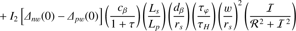
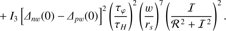


![$\displaystyle = \left[{\mit\Delta}_{nw}(0)-{\mit\Delta}_{pw}(0)\right]\left(\fr...
..._H^{\,2}\,\vert\omega_{\perp\,i}\vert}\right)\left(\frac{w_{pw}}{r_s}\right)^4,$](img3259.png)


![$\displaystyle = \left[{\mit\Delta}_{nw}(0)-{\mit\Delta}_{pw}(0)\right]\left(\fr...
..._H^{\,2}\,\vert\omega_{\perp\,i}\vert}\right)\left(\frac{w_{pw}}{r_s}\right)^4,$](img3312.png)