Next: Rotation Braking by a Up: Rotation Braking in Tokamak Previous: Introduction Contents
Assuming that the chain possesses the rotation frequency  in the laboratory frame, so that
 , and that
 (i.e., there is no error-field),
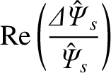
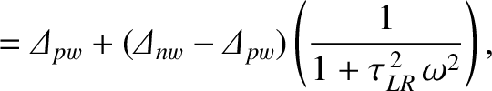
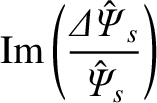
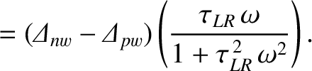
Equation (3.188) yields
(i.e., there is no error-field),
Equation (3.188) yields
 is the normalized reconnected magnetic flux at the rational surface [see Equations (3.72) and (3.184)],
 is the normalized helical magnetic flux that penetrates the
wall [see Equations (3.82) and (3.192)], the real dimensionless parameters
is the normalized helical magnetic flux that penetrates the
wall [see Equations (3.82) and (3.192)], the real dimensionless parameters  and
and
 are defined in Equations (3.87) and (3.195), respectively,
 |
(10.2) |
 time of the wall, and
  the time-constant of the wall [see Equation (3.103)].
Note that Equation (10.1) is only valid in the so-called thin-wall limit,
[see Equation (3.104)], where
the time-constant of the wall [see Equation (3.103)].
Note that Equation (10.1) is only valid in the so-called thin-wall limit,
[see Equation (3.104)], where  is the radial thickness of the wall, and
  its minor radius. The previous inequality ensures that the perturbed radial magnetic field only exhibits weak radial variation across the wall.
Equations (3.187) and (10.1) yield
 |
(10.4) |
 is the (real, dimensionless) tearing stability index when the wall is perfectly conducting (i.e.,
 ), whereas
 is the (real, dimensionless) tearing stability index when there is no wall (i.e.,
 ). We expect
 . In other words, we expect the magnetic island chain to
be stabilized by the presence of a perfectly conducting wall [3,10].
. In other words, we expect the magnetic island chain to
be stabilized by the presence of a perfectly conducting wall [3,10].
It follows from the previous equation that
 |
 |
(10.5) |
 |
 |
(10.6) |
 is the perfect-wall tearing stability index when the width of the magnetic island
chain at the rational surface is zero. Likewise,
is the perfect-wall tearing stability index when the width of the magnetic island
chain at the rational surface is zero. Likewise,
 is the no-wall tearing stability index when the width of the magnetic island
chain at the rational surface is zero. Finally,
is the no-wall tearing stability index when the width of the magnetic island
chain at the rational surface is zero. Finally,
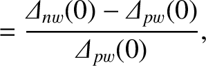
 , where
  is the saturated radial magnetic island width when the wall is perfectly conducting [see Equation (9.21)].
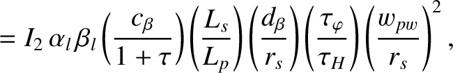
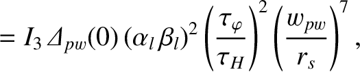
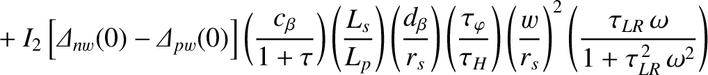
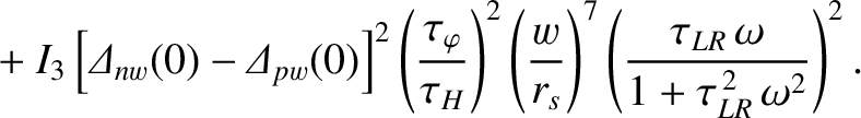
Equations (8.108), (10.7), and (10.8) yield the following modified Rutherford island width evolution equation [13]:
Here, is the minor radius of the rational surface,
  the resistive evolution time [see Equation (5.49)],
  the hydromagnetic time [see Equation (5.43)],
 the toroidal momentum confinement time [see Equation (5.50)],
  a dimensionless measure of the plasma pressure at the rational surface [see Equation (4.65)],
  the ratio of the electron and ion pressure gradients at the rational surface
[see Equation (4.5)],
the ratio of the electron and ion pressure gradients at the rational surface
[see Equation (4.5)],  the radial width of the magnetic island chain,
 the ion sound radius,
  the collisionless ion skin-depth at the rational surface [see Equation (4.24)],
  the magnetic shear-length at the rational surface [see Equation (5.27)], and
  the effective pressure gradient scale-length at the rational surface [see Equation (8.35)].
Furthermore,
the effective pressure gradient scale-length at the rational surface [see Equation (8.35)].
Furthermore,
 ,
,
 , and
, and
 . (See Section 8.11.)
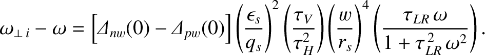
The first term on the right-hand side of the previous equation governs the growth and saturation of the magnetic island chain when its rotation frequency is sufficiently large that the wall acts as a perfect conductor. The second term describes the loss of wall stabilization when the chain's rotation frequency is sufficiently small that perturbed magnetic field can penetrate through the wall [3,10]. The third and fourth terms represent the destabilizing effect of the ion polarization current induced in the vicinity of the rational surface when the ion fluid is diverted around the island chain's magnetic separatrix [7,13]. Unlike the case of an isolated island chain (see Chapter 9), the polarization effect is non-zero because, according to Equation (8.74), (8.87), (8.101), and (10.8), the electromagnetic braking torque exerted on the plasma in the immediate vicinity of the rational surface, due to interaction with the conducting wall, generates finite ion flow in the island rest frame.
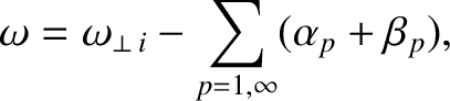
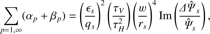
Assuming that the island chain co-rotates with the ion fluid at the rational surface (see Section 9.5), Equations (3.189) and (9.31) imply that
where , which is defined in Equation (9.32), is the unperturbed (by any electromagnetic torques that develop at the rational surface) rotation frequency. Here, we are treating
  and
and  as constants because the electromagnetic torque that develops at the rational surface has no explicit time
dependance (assuming that the width of the island chain grows on a timescale that is much greater than
as constants because the electromagnetic torque that develops at the rational surface has no explicit time
dependance (assuming that the width of the island chain grows on a timescale that is much greater than
 and
). Equations (3.180), (3.190), (3.191),
(4.23), (5.27), (5.43), (5.50), (7.28), and (7.34)–(7.35)
can be combined to give
where
Here,
and
). Equations (3.180), (3.190), (3.191),
(4.23), (5.27), (5.43), (5.50), (7.28), and (7.34)–(7.35)
can be combined to give
where
Here,
 is the poloidal flow-damping time [see Equation (7.28)],
 ,
,  the simulated major radius of the plasma,
  the minor radius of the plasma,
  ,
,  the poloidal mode number of the island chain, and
  the toroidal mode number of the island chain. Equations (10.8), (10.10), and (10.11) can be combined to give the
torque balance equation [6]
The left-hand side of the previous equation represents the viscous restoring torque that acts to prevent changes in the
plasma rotation at the rational surface, whereas the right-hand side represents the electromagnetic
braking torque acting on the plasma in the vicinity of the rational surface due to the eddy current induced in the conducting wall.
the toroidal mode number of the island chain. Equations (10.8), (10.10), and (10.11) can be combined to give the
torque balance equation [6]
The left-hand side of the previous equation represents the viscous restoring torque that acts to prevent changes in the
plasma rotation at the rational surface, whereas the right-hand side represents the electromagnetic
braking torque acting on the plasma in the vicinity of the rational surface due to the eddy current induced in the conducting wall.
![\includegraphics[width=1.\textwidth]{Chapter10/Figure10_1.eps}](img3050.png)
|
Let
 |
 |
(10.14) |
 |
 |
(10.15) |
 |
 |
(10.16) |
 is defined in Equation (9.22). Thus,
  is the width of the magnetic island chain relative to its saturated width when the wall is perfectly conducting,
  is the island
rotation frequency relative to its value when there is no interaction with the wall, and
is the island
rotation frequency relative to its value when there is no interaction with the wall, and  is time
normalized to the typical time required for the island chain to attain is final saturated width.
The modified Rutherford equation, (10.9), and the torque balance equation, (10.13), can be
written in the non-dimensional forms [13]
respectively,
where
is time
normalized to the typical time required for the island chain to attain is final saturated width.
The modified Rutherford equation, (10.9), and the torque balance equation, (10.13), can be
written in the non-dimensional forms [13]
respectively,
where
 |
 |
(10.19) |
 |
 |
(10.20) |
 |
 |
(10.21) |
 |
 |
(10.22) |
 |
![$\displaystyle = \left[{\mit\Delta}_{nw}(0)-{\mit\Delta}_{pw}(0)\right]\left(\fr...
...\frac{\tau_{LR}\,\tau_V}{\tau_H^{\,2}}\right)\left(\frac{w_{pw}}{r_s}\right)^4,$](img3069.png) |
(10.23) |
 .
Here, we have added artificial plasma inertia (i.e., the
.
Here, we have added artificial plasma inertia (i.e., the
 term) into the torque balance equation, (10.18), in order to distinguish between dynamically-stable and dynamically-unstable solutions [6].
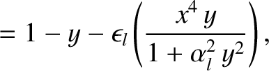
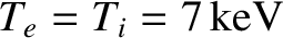
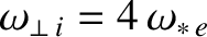
The steady-state solutions of the torque balance equation, (10.18), correspond to the roots of the cubic polynomial
 |
(10.24) |
 then the previous equation only possesses one real root. In this situation, the
normalized island rotation frequency, , slows down in a smooth reversible fashion as the
normalized island width, , increases [6]. On the other hand, if
then the previous equation only possesses one real root. In this situation, the
normalized island rotation frequency, , slows down in a smooth reversible fashion as the
normalized island width, , increases [6]. On the other hand, if
 then the
previous equation possesses three real roots. However, the intermediate root is dynamically unstable.
In this situation, the torque balance equation possesses two branches of dynamically-stable solutions [6]. The high-rotation
solution branch is characterized by
then the
previous equation possesses three real roots. However, the intermediate root is dynamically unstable.
In this situation, the torque balance equation possesses two branches of dynamically-stable solutions [6]. The high-rotation
solution branch is characterized by
 . On the other hand, the
low-rotation solution branch is characterized by
. On the other hand, the
low-rotation solution branch is characterized by
 .
The two solution branches are separated by a forbidden band of island rotation frequencies. The existence of this forbidden band has been verified experimentally [8].
The high-rotation solution branch ceases to exist when the normalized island width exceeds a critical
value, and there is a bifurcation to the low-rotation solution branch. Likewise, the low-rotation solution
branch ceases to exist when the normalized island width falls below a different critical value, and there is
a bifurcation to the high-rotation solution branch. Thus, if
then the slowing down
of the island rotation frequency with increasing island width is neither smooth nor reversible [6]. The steady-state solutions of the
torque balance equation are illustrated in Figure 10.1.
.
The two solution branches are separated by a forbidden band of island rotation frequencies. The existence of this forbidden band has been verified experimentally [8].
The high-rotation solution branch ceases to exist when the normalized island width exceeds a critical
value, and there is a bifurcation to the low-rotation solution branch. Likewise, the low-rotation solution
branch ceases to exist when the normalized island width falls below a different critical value, and there is
a bifurcation to the high-rotation solution branch. Thus, if
then the slowing down
of the island rotation frequency with increasing island width is neither smooth nor reversible [6]. The steady-state solutions of the
torque balance equation are illustrated in Figure 10.1.
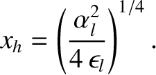
In the limit
 , we can find approximate solutions of the torque balance equation, (10.18).
The
high-rotation solution branch is characterized by
, we can find approximate solutions of the torque balance equation, (10.18).
The
high-rotation solution branch is characterized by
 , and is such that
![$\displaystyle y \simeq \frac{1}{2}\left(1+\left[1-\left(\frac{x}{x_h}\right)^4\right]^{1/2}\right),$](img3079.png) |
(10.25) |
 |
(10.26) |
, exceeds the
critical value,  —at which point the island rotation frequency has been reduced to half of its original value—and
there is a bifurcation to the low-rotation solution branch.
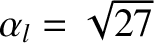
The low-rotation solution branch is characterized by
—at which point the island rotation frequency has been reduced to half of its original value—and
there is a bifurcation to the low-rotation solution branch.
The low-rotation solution branch is characterized by
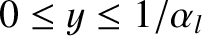 , and is such that
![$\displaystyle y \simeq \frac{1}{\alpha_l}\left\{\left(\frac{x}{x_l}\right)^4-\left[\left(\frac{x}{x_l}\right)^8-1\right]^{1/2}\right\},$](img3083.png) |
(10.27) |
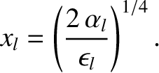 |
(10.28) |
 , and there is a bifurcation to the high-rotation solution branch. Note that
 , which indicates that, once the width of the
island chain has grown sufficiently wide to trigger a high-rotation to low-rotation bifurcation, the chain is unlikely to ever attain a
high-rotation state again (because its width would have to shrink by a considerable factor to trigger the reverse bifurcation).
In the limit
, the forbidden band of normalized island rotation frequencies corresponds to
, which indicates that, once the width of the
island chain has grown sufficiently wide to trigger a high-rotation to low-rotation bifurcation, the chain is unlikely to ever attain a
high-rotation state again (because its width would have to shrink by a considerable factor to trigger the reverse bifurcation).
In the limit
, the forbidden band of normalized island rotation frequencies corresponds to
 . (See Figure 10.1.)
![\includegraphics[width=\textwidth]{Chapter10/Figure10_2.eps}](img3088.png)
|
It is clear from Equation (10.17) that the slowing down of the island chain's rotation due to the eddy current induced in the conducting wall has a destabilizing effect on the chain. In fact, if there is no substantial slowing down then the normalized modified Rutherford equation (10.17) reduces to
 |
(10.29) |
 ,
,
 ,
,
 ,
indicating that the normalized island width, , saturates at its perfect-wall value, unity. On the other hand, on the low-rotation
solution branch, assuming that
and
,
indicating that the normalized island width, , saturates at its perfect-wall value, unity. On the other hand, on the low-rotation
solution branch, assuming that
and 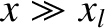 , Equation (10.17) reduces to
indicating that the normalized island width saturates at a value that is greater than unity. (Because
, Equation (10.17) reduces to
indicating that the normalized island width saturates at a value that is greater than unity. (Because  ,
,  ,
,  , and
, and
 are all positive quantities.) The island chain is
destabilized by the loss of wall stabilization, and also by the ion polarization effect associated with rotation braking.
are all positive quantities.) The island chain is
destabilized by the loss of wall stabilization, and also by the ion polarization effect associated with rotation braking.
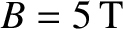
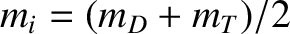
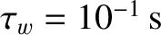
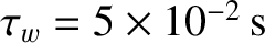
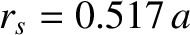
Figure 10.2 shows a numerical solution of Equations (10.17) and (10.18) made for
a low-field and a high-field tokamak fusion reactor. (See Chapter 1.) The simulation parameters are determined using the following assumptions:
 (low-field) or
 (high-field),
 ,
,
 ,
,
 (where
  and
and  are the deuteron and triton masses, respectively),
 ,
,  ,
,
 ,
,
 ,
,
 .
Here,
.
Here,
 is the electron diamagnetic frequency [see Equation (5.45)].
The poloidal and toroidal mode numbers of the magnetic island chain are
is the electron diamagnetic frequency [see Equation (5.45)].
The poloidal and toroidal mode numbers of the magnetic island chain are  are
are  ,
respectively. The wall parameters are
,
respectively. The wall parameters are
 and
and 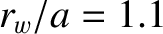 , which correspond to a moderately conducting, close-fitting wall. The plasma equilibrium is
assumed to be of the Wesson type (see Section 9.4), with
, which correspond to a moderately conducting, close-fitting wall. The plasma equilibrium is
assumed to be of the Wesson type (see Section 9.4), with 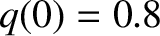 and
and  . It follows that
 . The perfect-wall saturated
island width is
. The perfect-wall saturated
island width is
 . Finally, the various dimensionless parameters appearing in Equations (10.17) and (10.18) take the values
 (low-field) or
 (high-field),
 ,
,
 ,
,
 ,
,
 , and
, and  .
.
It can be seen from Figure 10.2 that as the normalized width, , of the island chain grows in time, the chain's normalized rotation frequency, , is gradually reduced, until
it has been reduced to about half of its original value, at which point there is a sudden collapse in the
rotation frequency to a very low value. The collapse in the rotation frequency causes the
chain to be further destabilized due to the loss of wall stabilization, and ion polarization effects.
Consequently, the
final saturated width of the island chain is greater than the perfect-wall saturated island width (i.e.,  ).
Note that a low-field tokamak fusion reactor is more susceptible to rotation braking than a high-field
fusion reactor because of its lower diamagnetic frequency (see Table 6.1), and consequent lower ion fluid rotation.
The slowing-down curves shown in the figure are similar in form to those observed experimentally when a wide magnetic island chain interacts electromagnetically with a resistive wall in a toroidal confinement device [4].
).
Note that a low-field tokamak fusion reactor is more susceptible to rotation braking than a high-field
fusion reactor because of its lower diamagnetic frequency (see Table 6.1), and consequent lower ion fluid rotation.
The slowing-down curves shown in the figure are similar in form to those observed experimentally when a wide magnetic island chain interacts electromagnetically with a resistive wall in a toroidal confinement device [4].
![\includegraphics[width=1.\textwidth]{Chapter10/Figure10_3.eps}](img3113.png)
|
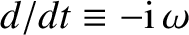
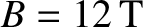
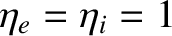
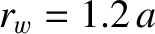
Figure 10.3 displays the results of a series of simulations of the type shown in Figure 10.2 in
which the radius of the rational surface is scanned over a range of values [by changing  while
keeping fixed]. The wall parameters are
while
keeping fixed]. The wall parameters are  and
and
 . It can be seen that if the rational surface lies well inside the plasma
boundary then the island chain attains its final, perfect-wall saturated width
without a collapse in its rotation frequency. On the other hand, if the rational surface lies closer to the plasma boundary then a collapse in the rotation frequency
is triggered before the chain attains its final saturated width. The critical island width at which the
rotation collapse is triggered lies between 20% and 10% of the plasma minor radius. Moreover, the final
saturated width of the island chain exceeds the perfect-wall value due to the loss of wall stabilization, and
ion polarization effects. Finally, it is again clear that a low-field tokamak fusion reactor is more susceptible to rotation braking than a high-field
fusion reactor.
. It can be seen that if the rational surface lies well inside the plasma
boundary then the island chain attains its final, perfect-wall saturated width
without a collapse in its rotation frequency. On the other hand, if the rational surface lies closer to the plasma boundary then a collapse in the rotation frequency
is triggered before the chain attains its final saturated width. The critical island width at which the
rotation collapse is triggered lies between 20% and 10% of the plasma minor radius. Moreover, the final
saturated width of the island chain exceeds the perfect-wall value due to the loss of wall stabilization, and
ion polarization effects. Finally, it is again clear that a low-field tokamak fusion reactor is more susceptible to rotation braking than a high-field
fusion reactor.
![\includegraphics[width=1.\textwidth]{Chapter10/Figure10_4.eps}](img3116.png)
|
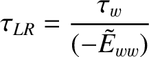
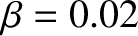
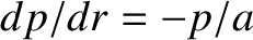
Figure 10.4 shows the results of a series of simulations of the type shown in Figure 10.2 in which
the
unperturbed island chain rotation frequency is scanned over a range of values for various different wall time-constants. The plasma parameters are
and 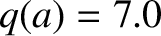 , which corresponds to
 , whereas the wall radius is
 .
It is clear that if the wall is very resistive (i.e.,
.
It is clear that if the wall is very resistive (i.e.,
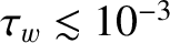 s) then the critical island width above which
the chain's rotation frequency collapses is only weakly dependent on the unperturbed rotation frequency, and
is about 10% of the plasma minor radius.
On the other hand, for the case of a highly conducting wall (i.e.,
s) then the critical island width above which
the chain's rotation frequency collapses is only weakly dependent on the unperturbed rotation frequency, and
is about 10% of the plasma minor radius.
On the other hand, for the case of a highly conducting wall (i.e.,
 s), diamagnetic
levels of plasma rotation are sufficient to completely suppress the collapse in the island rotation frequency, unless the unperturbed rotation
frequency lies close to zero. As before, it is clear that a low-field tokamak fusion reactor is more susceptible to rotation braking than a high-field
fusion reactor.
s), diamagnetic
levels of plasma rotation are sufficient to completely suppress the collapse in the island rotation frequency, unless the unperturbed rotation
frequency lies close to zero. As before, it is clear that a low-field tokamak fusion reactor is more susceptible to rotation braking than a high-field
fusion reactor.
![$\displaystyle = {\mit\Delta}_{pw}(0)\left(1-\frac{w}{w_{pw}}\right) + \left[{\m...
...-{\mit\Delta}_{pw}(0)\right]\left(\frac{1}{1+\tau_{LR}^{\,2}\,\omega^2}\right),$](img3028.png)
![$\displaystyle =\left[{\mit\Delta}_{nw}(0)-{\mit\Delta}_{pw}(0)\right]\left(\frac{\tau_{LR}\,\omega}{1+\tau_{LR}^{\,2}\,\omega^2}\right).$](img3029.png)
![$\displaystyle = {\mit\Delta}_{pw}(0)\left(1-\frac{w}{w_{pw}}\right) + \left[{\m...
...)-{\mit\Delta}_{pw}(0)\right]\left(\frac{1}{1+\tau_{LR}^{\,2}\,\omega^2}\right)$](img3033.png)
![$\displaystyle \tau_V = \frac{1}{4}\left[\left(\frac{q_s}{\epsilon_s}\right)^2\l...
...tau_\varphi}\right)^{1/2}
+2\,\ln\left(\frac{a}{r_s}\right)\right]\tau_\varphi.$](img3046.png)


![$\displaystyle = 1 - x +\beta_l\left(\frac{1}{1+\alpha_l^2\,y^2}\right) + \gamma...
...,y^2}\right)
+\delta_l \left[\frac{x^7\,y^2}{(1+\alpha_l^2\,y^2)^{\,2}}\right],$](img3057.png)