Next: Jeffries Connection Formula
Up: Wave Propagation in Inhomogeneous
Previous: Stokes Constants
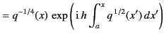
Let us write
 , where
  and
and  are real variables.
Consider the solution of the differential equation
are real variables.
Consider the solution of the differential equation
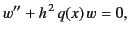 |
(1196) |
where  is a real function,
 is a large number,
  for
for  , and
, and  for
for  .
It is clear that
.
It is clear that  represents a simple zero of
 .
Here, we assume, as seems eminently reasonable,
that we can find a well-behaved function of the complex
variable
such that
.
Here, we assume, as seems eminently reasonable,
that we can find a well-behaved function of the complex
variable
such that
 along the real axis.
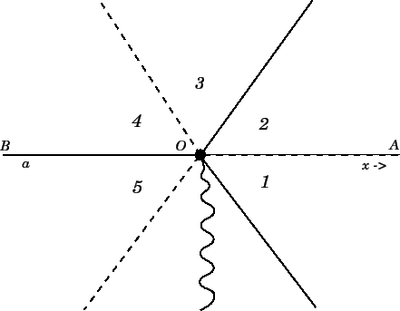
The arrangement of Stokes and anti-Stokes lines in the immediate vicinity
of the point
is sketched in Figure 24. The argument of
on
the positive
-axis is chosen to be
along the real axis.
The arrangement of Stokes and anti-Stokes lines in the immediate vicinity
of the point
is sketched in Figure 24. The argument of
on
the positive
-axis is chosen to be  . Thus, the argument of
on the negative
-axis is 0
.
. Thus, the argument of
on the negative
-axis is 0
.
Figure:
The
arrangement of Stokes lines (dashed) and anti-Stokes lines
(solid) in the complex  plane. Also shown is the branch
cut (wavy line).
plane. Also shown is the branch
cut (wavy line).
 |
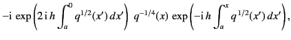
On  , the two WKB solutions (1176)-(1177) can be written
Here, we can interpret  as a wave propagating to the right along the
-axis, and
as a wave propagating to the right along the
-axis, and  as a wave propagating to the left.
On
as a wave propagating to the left.
On  , the WKB solutions take the form
Clearly,  represents an evanescent wave that decays to the right along the
-axis, whereas
represents an evanescent wave that decays to the right along the
-axis, whereas  represents an evanescent wave that decays to the
left. If we adopt the boundary condition that there is no incident wave from the
region
represents an evanescent wave that decays to the
left. If we adopt the boundary condition that there is no incident wave from the
region
 , the most general asymptotic solution to Equation (1198)
on
is written
, the most general asymptotic solution to Equation (1198)
on
is written
 |
(1201) |
where  is an arbitrary constant.
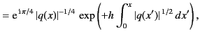
Let us assume that we can find an analytic solution,
 , to
the differential equation
, to
the differential equation
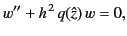 |
(1202) |
which satisfies
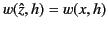 along the real axis, where
  is
the physical solution. From a mathematical point of view, this seems eminently
reasonable. In the domains 1 and 2, the solution (1203) becomes
is
the physical solution. From a mathematical point of view, this seems eminently
reasonable. In the domains 1 and 2, the solution (1203) becomes
 |
(1203) |
and
 |
(1204) |
respectively.
Note that the solution is continuous across the Stokes line
, because
the coefficient of the dominant solution
 is zero: thus, the
jump in the coefficient of the subdominant solution is zero times the
Stokes constant,
is zero: thus, the
jump in the coefficient of the subdominant solution is zero times the
Stokes constant,  . In other words, it is zero. Let us move into domain 3. In doing so,
we cross an anti-Stokes line, so the solution becomes
. In other words, it is zero. Let us move into domain 3. In doing so,
we cross an anti-Stokes line, so the solution becomes
 |
(1205) |
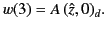
Let us now move into domain 4. In doing so, we cross a Stokes line. Applying the
general rule derived in the preceding section, the solution becomes
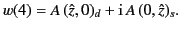 |
(1206) |
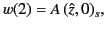
Finally, on
the solution becomes
 |
(1207) |
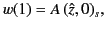
Suppose that there is a point  on the negative
-axis where
on the negative
-axis where  .
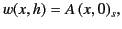
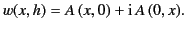
It follows from Equations (1201) and (1209) that we can write the asymptotic
solution to Equation (1198) as
.
It follows from Equations (1201) and (1209) that we can write the asymptotic
solution to Equation (1198) as
in the region
, and
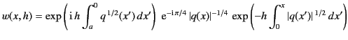 |
(1209) |
in the region
. Here, we have chosen
 |
(1210) |
If we interpret
as a normalized altitude in the ionosphere,
as the
square of the refractive index in the ionosphere, the point
as ground level,
and  as the electric field strength of a radio wave propagating vertically
upwards into the ionosphere, then Equation (1210) tells us that a unit amplitude
wave fired vertically upwards from ground level into the ionosphere
is reflected at the level where the refractive index is zero. The first term in
Equation (1210) is the incident wave, and the second term is the reflected wave.
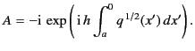
The reflection coefficient (i.e., the ratio of the reflected to the
incident wave at ground level) is given by
as the electric field strength of a radio wave propagating vertically
upwards into the ionosphere, then Equation (1210) tells us that a unit amplitude
wave fired vertically upwards from ground level into the ionosphere
is reflected at the level where the refractive index is zero. The first term in
Equation (1210) is the incident wave, and the second term is the reflected wave.
The reflection coefficient (i.e., the ratio of the reflected to the
incident wave at ground level) is given by
 |
(1211) |
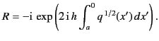
Note that  , so the amplitude of the reflected wave equals that of the
incident wave. In other words, there is no absorption of the wave at the level
of reflection. The phase shift of the reflected wave at ground level, with
respect to that of the incident wave, is that associated with the wave propagating
from ground level to the reflection level and back to ground level again,
plus a
, so the amplitude of the reflected wave equals that of the
incident wave. In other words, there is no absorption of the wave at the level
of reflection. The phase shift of the reflected wave at ground level, with
respect to that of the incident wave, is that associated with the wave propagating
from ground level to the reflection level and back to ground level again,
plus a  phase shift at reflection.
According to Equation (1211), the wave attenuates fairly rapidly
(in the space of a few wavelengths) above the reflection level. Of course,
Equation (1213) is completely equivalent to Equation (1089).
phase shift at reflection.
According to Equation (1211), the wave attenuates fairly rapidly
(in the space of a few wavelengths) above the reflection level. Of course,
Equation (1213) is completely equivalent to Equation (1089).
Note that the reflection of the incident
wave at the point where the refractive index is
zero is directly associated with the Stokes phenomenon. Without the jump
in the coefficient of the subdominant solution, as we go from domain 3 to domain 4,
there is no reflected wave on the
axis. Note, also, that the
WKB solutions (1210) and (1211) break down in the immediate vicinity
of  (i.e., at the reflection point). Thus, it is possible to
demonstrate
that the incident wave is totally reflected at the point
,
with a
phase shift,
without having to solve for the wave structure in the immediate vicinity
of the reflection point. This demonstrates that the reflection of the incident wave
at
is an intrinsic
property of the WKB solutions, and does not depend on the detailed behavior of the
wave in the region where the WKB solutions break down.
(i.e., at the reflection point). Thus, it is possible to
demonstrate
that the incident wave is totally reflected at the point
,
with a
phase shift,
without having to solve for the wave structure in the immediate vicinity
of the reflection point. This demonstrates that the reflection of the incident wave
at
is an intrinsic
property of the WKB solutions, and does not depend on the detailed behavior of the
wave in the region where the WKB solutions break down.
Next: Jeffries Connection Formula
Up: Wave Propagation in Inhomogeneous
Previous: Stokes Constants
Richard Fitzpatrick
2014-06-27