Next: Wave Propagation in Magnetized
Up: Wave Propagation in Uniform
Previous: Polarization of Electromagnetic Waves
Faraday Rotation
The electromagnetic force acting on an electron is given by
 |
(817) |
If the  and
and  fields in question
are due to an electromagnetic
wave propagating through a dielectric medium then
fields in question
are due to an electromagnetic
wave propagating through a dielectric medium then
 |
(818) |
where  is the refractive index.
It follows that the ratio of the magnetic to the electric forces acting on the
electron is
is the refractive index.
It follows that the ratio of the magnetic to the electric forces acting on the
electron is  . In other words, the magnetic force is
completely negligible
unless the wave amplitude is sufficiently high that the electron
moves relativistically in response to the wave. This state of affairs
is rare, but
can occur when
intense laser beams are made to propagate through plasmas.
. In other words, the magnetic force is
completely negligible
unless the wave amplitude is sufficiently high that the electron
moves relativistically in response to the wave. This state of affairs
is rare, but
can occur when
intense laser beams are made to propagate through plasmas.
Suppose, however, that the dielectric
medium contains an externally generated magnetic
field,
. This can easily be made much stronger than the optical
magnetic field. In this case, it is possible for a magnetic
field to affect the
propagation of low amplitude electromagnetic waves. The electron equation
of motion (779) generalizes to
 |
(819) |
where any damping of the motion
has been neglected. Let
be directed in the positive  -direction, and let the wave propagate in the
same direction. These assumptions imply that the
and
-direction, and let the wave propagate in the
same direction. These assumptions imply that the
and  vectors
lie in the
vectors
lie in the  -
- plane. The previous equation reduces to
provided that all perturbed quantities have an
 time dependence.
Here,
time dependence.
Here,
 , and
, and
 |
(822) |
is the electron cyclotron frequency.
Let
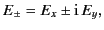 |
(823) |
and
 |
(824) |
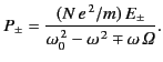
Note that
Equations (821) and (822) reduce to
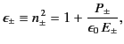
Defining
 , it follows from Equation (778)
that
, it follows from Equation (778)
that
 |
(829) |
Finally, from Equation (784), we can write
 |
(830) |
giving
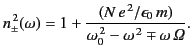 |
(831) |
According to the dispersion relation (832), the refractive index of a
magnetized dielectric medium can take one of
two possible values, which
presumably correspond to
two different types of wave propagating parallel to the
-axis. The
first wave has the refractive index  , and an associated electric
field [see Equations (826) and (827)]
, and an associated electric
field [see Equations (826) and (827)]
This corresponds to a left-hand circularly polarized wave
propagating in the
-direction at the phase velocity
 . The second wave has the refractive index
  , and an associated electric
field
, and an associated electric
field
This corresponds to a right-hand circularly polarized wave
propagating in the
-direction at the phase velocity
 . It is clear from Equation (832) that
  .
We conclude that, in the presence of a
-directed magnetic field,
a
-directed left-hand circularly polarized wave propagates at
a phase velocity that is slightly less than that of
the corresponding right-hand wave. It should be remarked that
the refractive index is always real (in the absence of damping), so the
magnetic field gives rise to no net absorption of electromagnetic
radiation. This is not surprising because a magnetic field does
no work on charged particles, and cannot therefore transfer energy from a wave propagating through a dielectric medium
to the medium's constituent particles.
.
We conclude that, in the presence of a
-directed magnetic field,
a
-directed left-hand circularly polarized wave propagates at
a phase velocity that is slightly less than that of
the corresponding right-hand wave. It should be remarked that
the refractive index is always real (in the absence of damping), so the
magnetic field gives rise to no net absorption of electromagnetic
radiation. This is not surprising because a magnetic field does
no work on charged particles, and cannot therefore transfer energy from a wave propagating through a dielectric medium
to the medium's constituent particles.
We have seen that right-hand and left-hand circularly polarized waves
propagate through a magnetized dielectric
medium at slightly different phase velocities. What does this imply for the propagation of a plane
polarized wave?
Let us add the left-hand wave whose electric field is given by
Equations (833) and (834) to the right-hand wave whose electric field is given by
Equations (835) and (836). In the absence of a magnetic field,  , and
we obtain
, and
we obtain
This, of course, corresponds to a plane wave
(polarized along the
-direction) propagating along the
-axis
at the phase velocity  . In the presence
of a magnetic field, we obtain
. In the presence
of a magnetic field, we obtain
where
 |
(840) |
is the mean index of refraction. Equations (839) and (840) describe
a plane wave whose angle of polarization with
respect to the
-axis,
 |
(841) |
rotates as the wave propagates along the
-axis at the
phase velocity
. In fact, the angle of polarization is given by
 |
(842) |
which clearly
increases linearly with the distance traveled by the wave parallel to the magnetic field.
This rotation of the plane
of polarization of a linearly polarized wave propagating through
a magnetized
dielectric medium is known as Faraday rotation (because it was
discovered by Michael Faraday in 1845).
Assuming that the cyclotron frequency,
 , is relatively small
compared to the wave frequency,
, is relatively small
compared to the wave frequency,  , and also that
does
not lie close to the resonant frequency,
, and also that
does
not lie close to the resonant frequency,  , it is easily
demonstrated that
, it is easily
demonstrated that
 |
(843) |
and
 |
(844) |
It follows that the rate at which the plane of polarization of
an electromagnetic wave rotates as the distance traveled by the
wave increases is
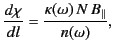 |
(845) |
where
 is the component of the magnetic field along the
direction of propagation of the wave,
and
is the component of the magnetic field along the
direction of propagation of the wave,
and
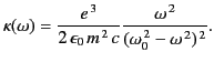 |
(846) |
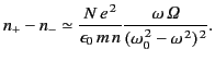
If the medium in question is a tenuous plasma then  , and
, and
 . Thus,
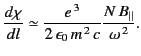 |
(847) |
In this case, the rate at which the plane of polarization rotates is
proportional to the product of the electron number density and the
parallel magnetic field-strength. Moreover, the plane of rotation
rotates faster for low frequency waves than for high frequency waves.
The total angle by which the plane of polarization is twisted
after passing through a magnetized plasma is given by
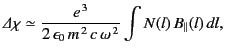 |
(848) |
assuming that  and
vary on length-scales that are
large compared to the wavelength of the radiation. This formula is
regularly employed in radio astronomy to infer the magnetic
field-strength in interstellar space.
and
vary on length-scales that are
large compared to the wavelength of the radiation. This formula is
regularly employed in radio astronomy to infer the magnetic
field-strength in interstellar space.
Next: Wave Propagation in Magnetized
Up: Wave Propagation in Uniform
Previous: Polarization of Electromagnetic Waves
Richard Fitzpatrick
2014-06-27