Wave Propagation in Magnetized Plasmas

For a plasma (in which $\omega_0=0$ ), the dispersion relation (832) reduces to

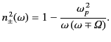$$n_\pm^{\,2}(\omega) = 1 - \frac{\omega_p^{\,2}}{\omega\,(\omega\mp{\mit \Omega})}.$$ (849)

The upper sign corresponds to a left-hand circularly polarized wave, and the lower sign to a right-hand polarized wave. Of course, Equation (850) is only valid for wave propagation parallel to the direction of the magnetic field. Wave propagation through the Earth's ionosphere is well described by the previous dispersion relation. There are wide frequency intervals where one of $n_+^{\,2}$ or $n_-^{\,2}$ is positive, and the other negative. At such frequencies, one state of circular polarization cannot propagate through the plasma. Consequently, a wave of that polarization incident on the plasma is totally reflected. (See Chapter 8). The other state of polarization is partially transmitted.

The behavior of $n^{\,2}_-(\omega)$ at low frequencies is responsible for a strange phenomenon known to radio hams as ``whistlers.'' As the wave frequency tends to zero, Equation (850) yields

$$n_-^{\,2} \simeq \frac{\omega_p^{\,2}}{\omega\,{\mit \Omega}}.$$ (850)

At such a frequency, $n_+^{\,2}$ is negative, so only right-hand polarized waves can propagate. The wavenumber of these waves is given by

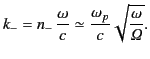$$k_- = n_-\,\frac{\omega}{c} \simeq\frac{\omega_p}{c} \sqrt{\frac{\omega}{\mit \Omega}}.$$ (851)

Now, energy propagates through a dispersive medium at the group velocity (see Section 7.13)

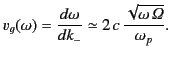$$v_g(\omega) = \frac{d\omega}{dk_-} \simeq 2\,c\, \frac{\sqrt{\omega\,{\mit\Omega}}}{\omega_p}.$$ (852)

Thus, low frequency waves transmit energy at a slower rate than high frequency waves. A lightning strike in one hemisphere of the Earth generates a wide spectrum of radiation, some of which propagates along the dipolar field-lines of the Earth's magnetic field in a manner described approximately by the dispersion relation (851). The high frequency components of the signal return to the surface of the Earth before the low frequency components (because they travel faster along the magnetic field). This gives rise to a radio signal that begins at a high frequency, and then ``whistles'' down to lower frequencies.