Next: Circular Current Loop
Up: Magnetostatic Fields
Previous: Biot-Savart Law
Making use of the fact that the magnetic fields generated by different current loops
are superposable (see Section 1.2), Equation (614) can easily be generalized to deal with the magnetic field
 generated by a continuous current
distribution of current density
generated by a continuous current
distribution of current density
 . In fact,
 |
(616) |
For the case of a steady (i.e.,
 ) current distribution, the charge conservation law (7) yields the constraint
 |
(617) |
Given that [see Equation (153)]
 |
(618) |
Equation (617) can also be written
 |
(619) |
where
 |
(620) |
Here,  is termed the vector potential. (See Section 1.3.)
It immediately follows that
is termed the vector potential. (See Section 1.3.)
It immediately follows that
 |
(621) |
which is the second Maxwell equation. (See Section 1.2.)
Now,
where we have integrated by parts, and neglected surface terms. Thus, according to Equation (618),
 |
(623) |
In other words, the vector potential defined in Equation (621) automatically satisfies the time independent version of the
Lorenz gauge condition, (13). Finally,
 |
(624) |
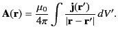
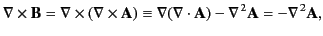
where use has been made of Equations (620) and (624). It follows from Equations (621) and (25) that
 |
(625) |
or
 |
(626) |
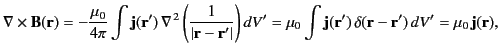
which is the time independent form of the fourth Maxwell equation. (See Section 1.2.) The integral version of the previous
equation, which follows from the curl theorem, is
 |
(627) |
This result is known as Ampère's law. Here,  is a closed curve spanned by a general surface
  .
.
Next: Circular Current Loop
Up: Magnetostatic Fields
Previous: Biot-Savart Law
Richard Fitzpatrick
2014-06-27