Next: Localized Current Distribution
Up: Magnetostatic Fields
Previous: Continuous Current Distribution
Let us calculate the magnetic field generated by a thin circular loop of radius  , lying in the
  -
- plane, centered on the origin, and carrying the steady current
  .
Let
.
Let  ,
,  ,
,  be spherical coordinates whose origin lies at the center of the loop, and whose symmetry axis is coincident with that
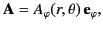
of the loop. It follows that the distribution of current density in space is
be spherical coordinates whose origin lies at the center of the loop, and whose symmetry axis is coincident with that
of the loop. It follows that the distribution of current density in space is
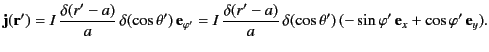 |
(628) |
Because the geometry is cylindrically symmetric, we can, without loss of generality, choose the observation point to lie in the
- plane (i.e.,
  ).
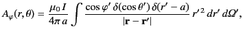
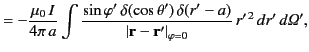
It follows from Equation (621) that
).
It follows from Equation (621) that
where
![$ \vert{\bf r}-{\bf r}'\vert _{\varphi=0} = [r^{\,2} + r'^{\,2}-2\,r\,r'\,(\cos\theta\,\cos\theta' + \sin\theta\,\sin\theta'\,\cos\varphi')]^{1/2}$](img1328.png) . It is clear that the integral for
. It is clear that the integral for  averages
to zero. Hence, only
averages
to zero. Hence, only  , which corresponds to
  , is non-zero, and we can write
 |
(632) |
where
 |
(633) |
which reduces to
 |
(634) |
The previous integral can be expressed in terms of complete elliptic integrals,![[*]](footnote.png) but this is not particularly illuminating.
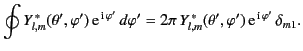
A better approach is to make use of the expansion of the Green's function for Poisson's equation in terms of spherical harmonics
given in Section 3.5:
but this is not particularly illuminating.
A better approach is to make use of the expansion of the Green's function for Poisson's equation in terms of spherical harmonics
given in Section 3.5:
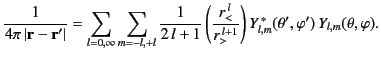 |
(635) |
Here,  represents the lesser of
and
represents the lesser of
and  , whereas
  represents the greater of
and
.
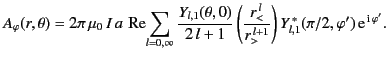
Hence,
represents the greater of
and
.
Hence,
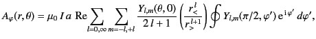 |
(636) |
where
now represents the lesser of
and
, whereas
represents the greater of
and
.
It follows from Equation (309) that
 |
(637) |
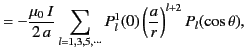
Thus, Equation (637) yields
 |
(638) |
However, according to Equation (309),
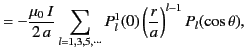
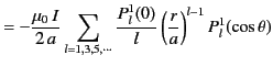
Hence, we obtain
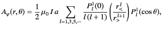 |
(641) |
where we have made use of the fact that
 when
when  is even.To be more exact,
 |
(642) |
for  , and
, and
 |
(643) |
for  .
.
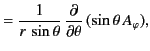
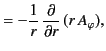
Now, according to Equations (620) and (633),
Given that
![$\displaystyle \frac{1}{\sin\theta}\,\frac{d}{d\theta}\left[\sin\theta\,P_l^1(\cos\theta)\right]=-l\,(l+1)\,P_l(\cos\theta),$](img1353.png) |
(647) |
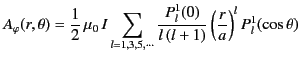
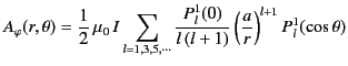
we find that
in the region
. In particular, because  and
and
 , we obtain
The previous two equations can be combined to give
 |
(652) |
Of course, this result can be obtained in a more straightforward fashion via the direct application of the Biot-Savart law.
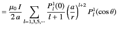
We also have
in the region
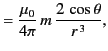
. A long way from the current loop (i.e.,
 ), we obtain
where
 .
.
Now, a small planar current loop of area  , carrying a current
, constitutes a magnetic dipole of moment
, carrying a current
, constitutes a magnetic dipole of moment
 |
(658) |
Here,  is a unit normal to the loop in the sense determined by the right-hand circulation rule (with the current determining the sense
of circulation). It follows that in the limit
is a unit normal to the loop in the sense determined by the right-hand circulation rule (with the current determining the sense
of circulation). It follows that in the limit
 and
and
 the current loop considered previously constitutes
a magnetic dipole of moment
the current loop considered previously constitutes
a magnetic dipole of moment
 . Moreover, Equations (656)-(658) specify the non-zero components
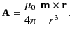
of the vector potential and the magnetic field generated by the dipole. It is easily seen from Equation (656) that
. Moreover, Equations (656)-(658) specify the non-zero components
of the vector potential and the magnetic field generated by the dipole. It is easily seen from Equation (656) that
 |
(659) |
Taking the curl of this expression, we obtain
![$\displaystyle {\bf B} =\frac{\mu_0}{4\pi}\left[\frac{3\,({\bf m}\cdot{\bf r})\,{\bf r} -r^{\,2}\,{\bf m}}{r^{\,5}}\right],$](img1378.png) |
(660) |
which is consistent with Equations (657) and (658).
Next: Localized Current Distribution
Up: Magnetostatic Fields
Previous: Continuous Current Distribution
Richard Fitzpatrick
2014-06-27
![$\displaystyle = \left[\frac{(2\,l+1)}{4\pi\,l\,(l+1)}\right]^{1/2}\,P_l^{\,1}(\cos\theta),$](img1340.png)
![$\displaystyle = \left[\frac{(2\,l+1)}{4\pi\,l\,(l+1)}\right]^{1/2}\,P_l^{\,1}(0).$](img1342.png)