Next: Boundary Value Problems
Up: Electrostatic Fields
Previous: Charge Sheets and Dipole
Green's Theorem
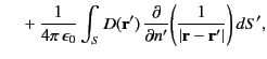
Consider the vector identity
 |
(216) |
where
 and
and
 are two arbitrary (but differentiable) vector fields. We can also
write
are two arbitrary (but differentiable) vector fields. We can also
write
 |
(217) |
Forming the difference between the previous two equation, we get
 |
(218) |
Finally, integrating this expression over some volume  , bounded by the closed surface
  , and making use
of the divergence theorem, we obtain
, and making use
of the divergence theorem, we obtain
 |
(219) |
This result is known as Green's theorem.
Changing the variable of integration, the above result can be rewritten
![$\displaystyle \int_V \left[\psi({\bf r}')\,\nabla'^{\,2}\phi({\bf r}')-\phi({\b...
...tial n'}-\phi({\bf r}')\,\frac{\partial\psi({\bf r}')}{\partial n'}\right] dS',$](img514.png) |
(220) |
where
 is shorthand for
 , et cetera.
Suppose that
is a solution to Poisson's equation,
, et cetera.
Suppose that
is a solution to Poisson's equation,
 |
(221) |
associated with some charge distribution,
 , that extends over all space,
subject to the boundary condition
, that extends over all space,
subject to the boundary condition
 as as  |
(222) |
Suppose, further, that
 |
(223) |
It follows from Equation (25), and symmetry, that
 |
(224) |
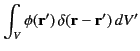
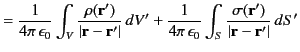
The previous five equations can be combined to give
where
It follows, by comparison with Equations (162), (202), and (205), that the three terms on the right-hand side of
Equation (225) are the electric potential generated by the charges distributed within
, the
potential generated by the surface charge distribution,
 , on
, and the potential generated by the surface dipole distribution,
, on
, and the potential generated by the surface dipole distribution,
 , on
, respectively.
, on
, respectively.
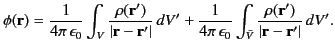
Suppose that the point  lies within
. In this case, Equation (225) yields
lies within
. In this case, Equation (225) yields
 |
(228) |
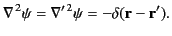
However, we know that the general solution to Equation (221), subject to the boundary condition (222), is
 |
(229) |
Here,
denotes the region of space lying within the closed surface
, whereas
 denotes the region
lying outside
. A comparison of the previous two equations reveals that, for a point
lying
within
,
denotes the region
lying outside
. A comparison of the previous two equations reveals that, for a point
lying
within
,
 |
(230) |
In other words, the electric potential (and, hence, the electric field) generated within
by the charges external to
is equivalent
to that generated by the charge sheet
, and the dipole sheet
, distributed on
. Furthermore, because  depends on
the normal derivative of the potential at
, whereas
depends on
the normal derivative of the potential at
, whereas  depends on the potential at
, it follows that we can completely determine
the potential within
once we known the distribution of charges within
, and the values of the potential and
its normal derivative on
. In fact, this is an overstatement, because the potential and its normal derivative are not independent
of one another, but are related via Poisson's equation. In other words, a knowledge of the potential on
also implies a knowledge of its
normal derivative, and vice versa. Hence, we can, actually, determine the potential within
from a knowledge of the distribution of charges inside
, and the distribution of either the potential, or its normal derivative, on
. The specification of the potential on
is
known as a Dirichlet boundary condition. On the other hand, the specification of the normal derivative of the
potential on
is called a Neumann boundary condition.
depends on the potential at
, it follows that we can completely determine
the potential within
once we known the distribution of charges within
, and the values of the potential and
its normal derivative on
. In fact, this is an overstatement, because the potential and its normal derivative are not independent
of one another, but are related via Poisson's equation. In other words, a knowledge of the potential on
also implies a knowledge of its
normal derivative, and vice versa. Hence, we can, actually, determine the potential within
from a knowledge of the distribution of charges inside
, and the distribution of either the potential, or its normal derivative, on
. The specification of the potential on
is
known as a Dirichlet boundary condition. On the other hand, the specification of the normal derivative of the
potential on
is called a Neumann boundary condition.
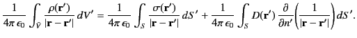
Suppose that the point
lies outside
. In this case, Equation (225) yields
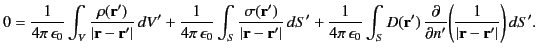 |
(231) |
In other words, outside
, the electric potential generated by the surface charge distribution
, combined with that generated by the surface dipole distribution
, completely
cancels out the electric potential (and, hence, the electric field) produced by the
charges distributed within
. As an example of this type of cancellation, suppose that
is a spherical surface of radius  , centered on the
origin. Within
, let there be a single charge
, centered on the
origin. Within
, let there be a single charge  , located at the origin.
The electric field and potential generated by this charge are
, located at the origin.
The electric field and potential generated by this charge are
 |
(232) |
and
 |
(233) |
respectively. It follows from Equations (226) and (227) that the densities of the charge and dipole sheets at  that are needed to cancel out the effect of the central charge in the region
  are
are
respectively. Making use of Equations (212)-(215), and (232)-(235), the electric field and
potential generated by the combination of the charge at the origin, the charge sheet at
, and the dipole sheet at
,
are
![$\displaystyle {\bf E} = \left\{ \begin{array}{lll} [q/(4\pi\,\epsilon_0\,r^{\,2...
...,{\bf e}_r&\mbox{\hspace{0.5cm}}& r<a\\ [0.5ex] {\bf0}&&r>a \end{array}\right.,$](img539.png) |
(236) |
and
![$\displaystyle \phi = \left\{ \begin{array}{lll} q/(4\pi\,\epsilon_0\,r)&\mbox{\hspace{0.5cm}}& r<a\\ [0.5ex] 0&&r>a \end{array}\right.,$](img540.png) |
(237) |
respectively. We can see that the charge and dipole sheet at
do not affect the electric field, or the potential, due to the central charge in the region  , but completely
cancel out this charge's field and potential in the region
.
, but completely
cancel out this charge's field and potential in the region
.
Next: Boundary Value Problems
Up: Electrostatic Fields
Previous: Charge Sheets and Dipole
Richard Fitzpatrick
2014-06-27