Next: Poisson's equation
Up: Time-independent Maxwell equations
Previous: The electric scalar potential
Gauss' law
Figure 26:
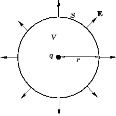 |
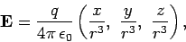
Consider a single charge located at the origin. The electric field generated by
such a charge is given by Eq. (171). Suppose that we surround the charge by
a concentric spherical surface  of radius
  (see Fig. 26). The flux of the
electric field through this surface is
given by
(see Fig. 26). The flux of the
electric field through this surface is
given by
 |
(187) |
since the normal to the surface is always
parallel to the local electric field.
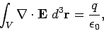
However, we also know from Gauss' theorem that
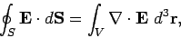 |
(188) |
where  is the volume enclosed by surface . Let us evaluate
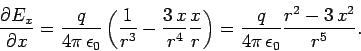
 directly. In Cartesian coordinates, the field is written
 |
(189) |
where
 . So,
. So,
 |
(190) |
Here, use has been made of
 |
(191) |
Formulae analogous to Eq. (190) can be obtained for
 and
and
 .
The divergence of the field is thus given by
.
The divergence of the field is thus given by
 |
(192) |
This is a puzzling result! We have from Eqs. (187) and (188) that
 |
(193) |
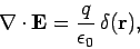
and yet we have just proved that
 . This paradox can be
resolved after a close examination of Eq. (192). At the origin
(
. This paradox can be
resolved after a close examination of Eq. (192). At the origin
( ) we find that
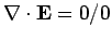 , which means that
can take any value at this point.
Thus, Eqs. (192) and (193) can be reconciled
if
is some sort
of ``spike'' function: i.e., it is zero everywhere except arbitrarily
close to the origin,
where it becomes very large. This
must occur in such a manner that the volume integral over the spike
is finite.
, which means that
can take any value at this point.
Thus, Eqs. (192) and (193) can be reconciled
if
is some sort
of ``spike'' function: i.e., it is zero everywhere except arbitrarily
close to the origin,
where it becomes very large. This
must occur in such a manner that the volume integral over the spike
is finite.
Figure 27:
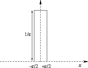 |
Let us examine how we might construct a one-dimensional spike function.
Consider the ``box-car'' function
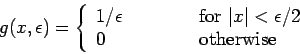 |
(194) |
(see Fig. 27).
It is clear that that
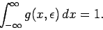 |
(195) |
Now consider the function
 |
(196) |
This is zero everywhere except arbitrarily close to  .
According to Eq. (195),
it also possess a finite integral;
.
According to Eq. (195),
it also possess a finite integral;
 |
(197) |
Thus,  has all of the required properties of a spike function.
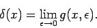
The one-dimensional spike function is called the
Dirac delta-function after the Cambridge physicist Paul Dirac who
invented it in 1927 while investigating quantum mechanics. The delta-function is an
example of what mathematicians call a generalized function: it is not
well-defined at , but its integral is nevertheless well-defined.
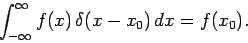
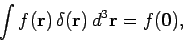
Consider the integral
has all of the required properties of a spike function.
The one-dimensional spike function is called the
Dirac delta-function after the Cambridge physicist Paul Dirac who
invented it in 1927 while investigating quantum mechanics. The delta-function is an
example of what mathematicians call a generalized function: it is not
well-defined at , but its integral is nevertheless well-defined.
Consider the integral
 |
(198) |
where  is a function which is well-behaved in the vicinity of .
Since the delta-function is zero everywhere apart from very close
to , it is clear that
is a function which is well-behaved in the vicinity of .
Since the delta-function is zero everywhere apart from very close
to , it is clear that
 |
(199) |
where use has been made of Eq. (197). The above equation, which is valid for any
well-behaved
function, , is effectively the definition of a delta-function.
A simple change of variables allows us to define  , which is
a spike function centred on
, which is
a spike function centred on  . Equation (199) gives
 |
(200) |
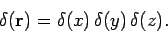
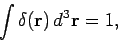
We actually want a three-dimensional spike function:
i.e., a function
which is zero everywhere
apart from arbitrarily close to the origin, and whose volume integral is unity.
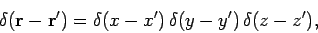
If we denote this function by
 then it is easily seen that
the three-dimensional delta-function is the product of three one-dimensional
delta-functions:
then it is easily seen that
the three-dimensional delta-function is the product of three one-dimensional
delta-functions:
 |
(201) |
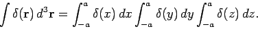
This function is clearly zero everywhere except the origin. But is its volume
integral unity? Let us integrate over a cube of dimensions  which is
centred on the origin, and aligned along the Cartesian axes. This
volume integral is obviously separable, so that
which is
centred on the origin, and aligned along the Cartesian axes. This
volume integral is obviously separable, so that
 |
(202) |
The integral can be turned into an integral over all space by taking
the limit
 . However, we know that for one-dimensional
delta-functions
. However, we know that for one-dimensional
delta-functions
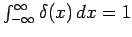 , so it follows
from the above equation that
, so it follows
from the above equation that
 |
(203) |
which is the desired result. A simple generalization of previous arguments yields
 |
(204) |
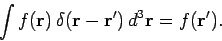
where  is any well-behaved scalar field. Finally, we can change variables
and write
is any well-behaved scalar field. Finally, we can change variables
and write
 |
(205) |
which is a three-dimensional spike function centred on
 . It is easily demonstrated that
 |
(206) |
Up to now, we have only considered volume integrals taken
over all space. However, it
should be obvious that the above result also holds for integrals
over any finite volume which contains the point
. Likewise,
the integral is zero if does not contain
.
Let us now return to the problem in hand. The electric field generated by a charge
 located at the origin has
everywhere apart from the
origin, and also satisfies
located at the origin has
everywhere apart from the
origin, and also satisfies
 |
(207) |
for a spherical volume centered on the origin. These two facts imply that
 |
(208) |
where use has been made of Eq. (203).
At this stage, vector field theory has yet to show its worth..
After all, we have just spent an inordinately long time proving something using
vector field theory which we
previously proved in one line [see Eq. (187)] using conventional
analysis. It is time to demonstrate the power of vector field theory.
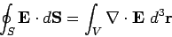
Consider, again, a charge at the origin surrounded by a spherical surface
which is centered on the origin.
Suppose that we now displace the surface , so that it is no longer centered
on the origin. What is the flux of the electric field out of S? This is not
a simple problem for conventional analysis, because the normal to the surface is
no longer parallel to the local electric field. However, using vector field theory
this problem is no more difficult than the previous one. We have
 |
(209) |
from Gauss' theorem,
plus Eq. (208).
From these equations,
it is clear that the flux of  out of is
  for a
spherical surface displaced from the origin. However, the flux becomes zero when the
displacement is sufficiently large that the origin is no longer enclosed by
the sphere.
It is possible to prove this via conventional analysis, but it is certainly not easy.
Suppose that the surface is not spherical but is
instead highly distorted. What now is the flux of out of ? This
is a virtually impossible problem in conventional analysis, but it is still easy
using vector field theory. Gauss' theorem and Eq. (208) tell us that
the flux is provided that the surface contains the origin,
and that the flux is zero otherwise. This result is completely independent of the shape of .
for a
spherical surface displaced from the origin. However, the flux becomes zero when the
displacement is sufficiently large that the origin is no longer enclosed by
the sphere.
It is possible to prove this via conventional analysis, but it is certainly not easy.
Suppose that the surface is not spherical but is
instead highly distorted. What now is the flux of out of ? This
is a virtually impossible problem in conventional analysis, but it is still easy
using vector field theory. Gauss' theorem and Eq. (208) tell us that
the flux is provided that the surface contains the origin,
and that the flux is zero otherwise. This result is completely independent of the shape of .
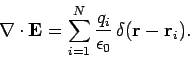
Consider  charges
  located at
  . A simple generalization of
Eq. (208) gives
. A simple generalization of
Eq. (208) gives
 |
(210) |
Thus, Gauss' theorem (209) implies that
 |
(211) |
where  is the total charge enclosed by the surface . This result is called
Gauss' law, and does
not depend on the shape of the surface.
is the total charge enclosed by the surface . This result is called
Gauss' law, and does
not depend on the shape of the surface.
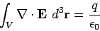
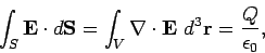
Suppose, finally, that instead of having a set of discrete charges, we have a
continuous charge distribution described by a charge density  .
The charge contained in a small rectangular volume of dimensions
.
The charge contained in a small rectangular volume of dimensions  ,
,  , and
, and  located at position
 is
is
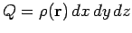 . However, if we integrate
over this volume element we obtain
. However, if we integrate
over this volume element we obtain
 |
(212) |
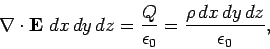
where use has been made of Eq. (211). Here, the volume element is assumed to be
sufficiently small that
does not vary significantly across
it. Thus, we obtain
 |
(213) |
This is the first of four field equations, called Maxwell's equations, which
together form
a complete description of electromagnetism. Of course, our derivation of
Eq. (213) is only valid for electric fields generated by stationary
charge distributions. In principle, additional terms might be required to describe
fields generated by moving charge distributions. However,
it turns out that this is not the case,
and that Eq. (213) is universally valid.
Equation (213) is a differential equation describing the electric field generated
by a set of charges. We already know the solution to this equation when the
charges are stationary:
it is given by Eq. (172),
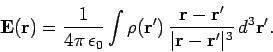 |
(214) |
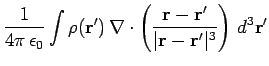
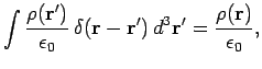
Equations (213) and (214) can be reconciled provided
 |
(215) |
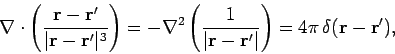
where use has been made of Eq. (175).
It follows that
which is the desired result. The most general form of Gauss' law, Eq. (211),
is obtained by integrating Eq. (213) over a volume surrounded by
a surface , and making use of
Gauss' theorem:
 |
(217) |
One particularly interesting application of Gauss' law is Earnshaw's
theorem, which states that it is impossible for a collection of charged particles to
remain in static equilibrium solely under the influence of electrostatic forces.
For instance, consider the motion of the  th particle in the
electric field, , generated by all of the other static particles.
The equilibrium position of the th particle corresponds to some
point , where
th particle in the
electric field, , generated by all of the other static particles.
The equilibrium position of the th particle corresponds to some
point , where
 . By implication,
does not correspond to the equilibrium position of
any other particle.
However, in order
for to be a stable equilibrium point, the particle
must experience a restoring force when it is moved a small
distance away from in any direction. Assuming that the
th particle is positively charged, this means that the electric
field must point radially towards
at all neighbouring points. Hence, if we apply Gauss' law to a small
sphere centred on , then there must be a negative flux of
through the surface of the sphere, implying the presence of a negative
charge at . However, there is no such charge at .
Hence, we conclude that cannot point radially towards
at all neighbouring points. In other
words, there must be some neighbouring points at which is directed away
from . Hence, a positively charged particle
placed at can always escape by moving to such points.
One corollary of Earnshaw's theorem is that classical electrostatics cannot
account for the stability of atoms and molecules.
. By implication,
does not correspond to the equilibrium position of
any other particle.
However, in order
for to be a stable equilibrium point, the particle
must experience a restoring force when it is moved a small
distance away from in any direction. Assuming that the
th particle is positively charged, this means that the electric
field must point radially towards
at all neighbouring points. Hence, if we apply Gauss' law to a small
sphere centred on , then there must be a negative flux of
through the surface of the sphere, implying the presence of a negative
charge at . However, there is no such charge at .
Hence, we conclude that cannot point radially towards
at all neighbouring points. In other
words, there must be some neighbouring points at which is directed away
from . Hence, a positively charged particle
placed at can always escape by moving to such points.
One corollary of Earnshaw's theorem is that classical electrostatics cannot
account for the stability of atoms and molecules.
Next: Poisson's equation
Up: Time-independent Maxwell equations
Previous: The electric scalar potential
Richard Fitzpatrick
2006-02-02