


Next: Summary
Up: Vectors
Previous: The Laplacian
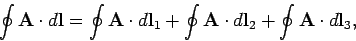
Consider a vector field  , and a loop which lies in one plane.
The integral of around this loop is written
, and a loop which lies in one plane.
The integral of around this loop is written
 , where
  is a line element of the
loop. If is a conservative field then
is a line element of the
loop. If is a conservative field then
 and
and
 for all loops. In general, for a non-conservative field,
 .
.
For a small loop we expect
to be proportional to
the area of the loop. Moreover, for a fixed area loop we expect
to depend on the orientation of the loop.
One particular orientation will give the maximum value:
 . If the loop subtends an angle
  with this optimum orientation
then we expect
with this optimum orientation
then we expect
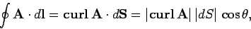
 . Let us introduce the vector field
 whose magnitude is
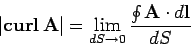 |
(143) |
for the orientation giving  . Here,
  is the area of the loop.
The direction of
is perpendicular to the plane of the loop,
when it is
in the
orientation giving , with the sense given by the right-hand grip rule.
is the area of the loop.
The direction of
is perpendicular to the plane of the loop,
when it is
in the
orientation giving , with the sense given by the right-hand grip rule.
Figure 22:
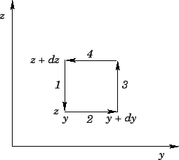 |
Let us now express
in terms of the components of .
First, we shall
evaluate
around a small rectangle in the
 -
- plane (see Fig. 22).
The contribution from sides 1 and 3 is
plane (see Fig. 22).
The contribution from sides 1 and 3 is
 |
(144) |
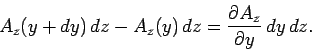
The contribution from sides 2 and 4 is
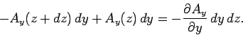 |
(145) |
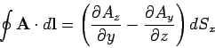
So, the total of all contributions gives
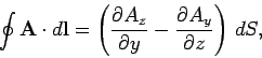 |
(146) |
where  is the area of the loop.
Consider a non-rectangular (but still small) loop in the - plane.
We can divide it into rectangular
elements, and form
over all the resultant
loops. The interior
contributions cancel, so we are just left with the contribution from the outer loop.
Also, the area of the outer loop is the sum of all the areas of the inner loops.
We conclude that
 |
(147) |
is valid for a small loop
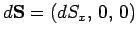 of any shape in the - plane. Likewise, we can show that
if the loop is in the
of any shape in the - plane. Likewise, we can show that
if the loop is in the  - plane then
 and
and
 |
(148) |
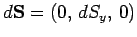
Finally, if the loop is in the - plane then
 and
and
 |
(149) |
Figure 23:
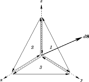 |
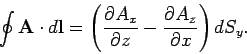
Imagine an arbitrary loop of vector area
 . We
can construct this out of three loops in the -, -, and -directions, as
indicated in Fig. 23.
If we form the line integral around all three loops then the interior contributions
cancel, and we are left with the line integral around the original loop. Thus,
. We
can construct this out of three loops in the -, -, and -directions, as
indicated in Fig. 23.
If we form the line integral around all three loops then the interior contributions
cancel, and we are left with the line integral around the original loop. Thus,
 |
(150) |
giving
 |
(151) |
where
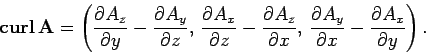 |
(152) |
Note that
 |
(153) |
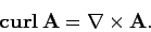
This demonstrates that
is a good vector field, since it is
the cross product of the  operator (a good vector operator) and
the vector field .
operator (a good vector operator) and
the vector field .
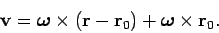
Consider a solid body rotating about the -axis. The angular velocity is given
by
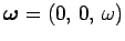 , so the rotation velocity at
position
, so the rotation velocity at
position  is
is
 |
(154) |
[see Eq. (43)].
Let us evaluate
 on the axis of
rotation. The -component is proportional to the
integral
on the axis of
rotation. The -component is proportional to the
integral
 around a loop in the - plane. This is
plainly zero. Likewise, the -component is also zero. The -component
is
around a loop in the - plane. This is
plainly zero. Likewise, the -component is also zero. The -component
is
 around some loop in the - plane.
Consider a circular loop. We have
around some loop in the - plane.
Consider a circular loop. We have
 with
with
 .
Here,
.
Here,  is the radial distance from the rotation axis.
It follows that
is the radial distance from the rotation axis.
It follows that
 , which
is independent of . So, on the axis,
, which
is independent of . So, on the axis,
 .
Off the axis, at position
.
Off the axis, at position  , we can write
 |
(155) |
The first part has the same curl as the velocity field on the axis, and the
second part has zero curl, since it is constant. Thus,
everywhere in the body. This allows us to
form a physical picture of
. If we imagine as the
velocity field of some fluid, then
at any given point is equal
to twice the local angular rotation velocity:
i.e., 2 .
Hence, a vector field with
.
Hence, a vector field with
 everywhere is said to
be irrotational.
everywhere is said to
be irrotational.
Another important result of vector field theory is the curl theorem
or Stokes' theorem,
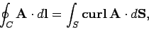 |
(156) |
for some (non-planar) surface  bounded by a rim
  . This theorem can easily
be proved by splitting the loop up into many small rectangular loops, and forming
the integral around all of the resultant loops. All of the contributions from the
interior loops cancel, leaving just the contribution from the outer rim.
Making use of Eq. (151) for each of the small loops, we can see that the contribution
from all of the loops is also equal to the integral of
. This theorem can easily
be proved by splitting the loop up into many small rectangular loops, and forming
the integral around all of the resultant loops. All of the contributions from the
interior loops cancel, leaving just the contribution from the outer rim.
Making use of Eq. (151) for each of the small loops, we can see that the contribution
from all of the loops is also equal to the integral of
 across the whole surface. This proves the theorem.
One immediate consequence of of Stokes' theorem is that
is ``incompressible.'' Consider two surfaces,  and
and  , which share the
same rim. It is clear from Stokes' theorem that
, which share the
same rim. It is clear from Stokes' theorem that
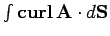 is the same for both surfaces. Thus, it
follows that
is the same for both surfaces. Thus, it
follows that
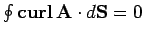 for any closed surface.
However, we have from the divergence theorem that
for any closed surface.
However, we have from the divergence theorem that
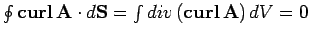 for any volume. Hence,
 |
(157) |
So,
 is a solenoidal field.
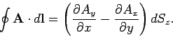
We have seen that for a conservative field
for any loop. This is entirely equivalent to
.
However, the magnitude of
is
 for some
particular loop. It is clear then that
for a conservative field. In other words,
for some
particular loop. It is clear then that
for a conservative field. In other words,
 |
(158) |
Thus, a conservative field is also an irrotational one.
Finally, it can be shown that
 |
(159) |
where
 |
(160) |
It should be emphasized, however, that the above result is only valid in
Cartesian coordinates.
Next: Summary
Up: Vectors
Previous: The Laplacian
Richard Fitzpatrick
2006-02-02