The Laplacian

So far we have encountered

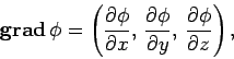$${\bf grad} \phi = \left(\frac{\partial \phi}{\partial x}, ... ...\phi} {\partial y}, \frac{\partial \phi}{\partial z}\right),$$ (131)

which is a vector field formed from a scalar field, and

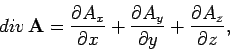$${\mit div} {\bf A} = \frac{\partial A_x}{\partial x} + \frac{\partial A_y}{\partial y} +\frac{\partial A_z}{\partial z},$$ (132)

which is a scalar field formed from a vector field. There are two ways in which we can combine ${\bf grad}$ and div. We can either form the vector field ${\bf grad} ({\mit div} {\bf A})$ or the scalar field ${\mit div} ({\bf grad} \phi)$. The former is not particularly interesting, but the scalar field ${\mit div} ({\bf grad} \phi)$ turns up in a great many physics problems, and is, therefore, worthy of discussion.

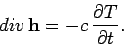
Let us introduce the heat flow vector ${\bf h}$, which is the rate of flow of heat energy per unit area across a surface perpendicular to the direction of ${\bf h}$. In many substances, heat flows directly down the temperature gradient, so that we can write

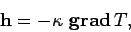$${\bf h} = - \kappa {\bf grad} T,$$ (133)

where $\kappa$ is the thermal conductivity. The net rate of heat flow $\oint_S {\bf h}\cdot d{\bf S}$ out of some closed surface $S$ must be equal to the rate of decrease of heat energy in the volume $V$ enclosed by $S$. Thus, we can write

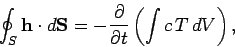$$\oint_S {\bf h}\cdot d{\bf S} = - \frac{\partial}{\partial t}\left( \int c T dV\right),$$ (134)

where $c$ is the specific heat. It follows from the divergence theorem that

$${\mit div} {\bf h} = -c \frac{\partial T}{\partial t}.$$ (135)

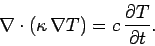
Taking the divergence of both sides of Eq. (133), and making use of Eq. (135), we obtain

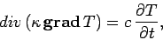$${\mit div}\left(\kappa {\bf grad} T\right) = c \frac{\partial T}{\partial t},$$ (136)

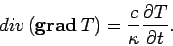
or

$${\nabla}\cdot\left(\kappa \nabla T\right) = c \frac{\partial T}{\partial t}.$$ (137)

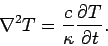
If $\kappa$ is constant then the above equation can be written

$${\mit div} ({\bf grad} T) = \frac{c}{\kappa} \frac{ \partial T}{\partial t}.$$ (138)

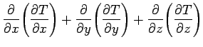
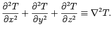
The scalar field ${\mit div} ({\bf grad} T)$ takes the form

$${\mit div} ({\bf grad} T) = \frac{\partial}{\partial x}\!\left(\frac{\partial T}{\partial x}\... ...right)+ \frac{\partial}{\partial z}\!\left(\frac{\partial T}{\partial z}\right)$$

$$= \frac{\partial^2 T}{\partial x^2}+\frac{\partial^2 T}{\partial y^2} + \frac{\partial^2 T}{\partial z^2} \equiv \nabla^2 T.$$ (139)

Here, the scalar differential operator

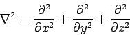$$\nabla^2 \equiv \frac{\partial^2}{\partial x^2}+ \frac{\partial^2}{\partial y^2}+ \frac{\partial^2}{\partial z^2}$$ (140)

is called the Laplacian. The Laplacian is a good scalar operator (i.e., it is coordinate independent) because it is formed from a combination of div (another good scalar operator) and ${\bf grad}$ (a good vector operator).

What is the physical significance of the Laplacian? In one dimension, $\nabla^2 T$ reduces to $\partial^2 T/\partial x^2$. Now, $\partial^2 T/\partial x^2$ is positive if $T(x)$ is concave (from above) and negative if it is convex. So, if $T$ is less than the average of $T$ in its surroundings then $\nabla^2 T$ is positive, and vice versa.

In two dimensions,

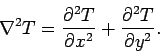$$\nabla^2 T = \frac{\partial^2 T}{\partial x^2}+ \frac{\partial ^2 T}{\partial y^2}.$$ (141)

Consider a local minimum of the temperature. At the minimum, the slope of $T$ increases in all directions, so $\nabla^2 T$ is positive. Likewise, $\nabla^2 T$ is negative at a local maximum. Consider, now, a steep-sided valley in $T$. Suppose that the bottom of the valley runs parallel to the $x$-axis. At the bottom of the valley $\partial^2 T/\partial y^2$ is large and positive, whereas $\partial^2 T/\partial x^2$ is small and may even be negative. Thus, $\nabla^2 T$ is positive, and this is associated with $T$ being less than the average local value.

Let us now return to the heat conduction problem:

$$\nabla^2 T = \frac{c}{\kappa} \frac{\partial T}{\partial t}.$$ (142)

It is clear that if $\nabla^2 T$ is positive then $T$ is locally less than the average value, so $\partial T/\partial t>0$: i.e., the region heats up. Likewise, if $\nabla^2 T$ is negative then $T$ is locally greater than the average value, and heat flows out of the region: i.e., $\partial T/\partial t<0$. Thus, the above heat conduction equation makes physical sense.