


Next: Divergence
Up: Vectors
Previous: Volume integrals
A one-dimensional function  has a gradient
  which is
defined as the slope of the tangent to the curve at
which is
defined as the slope of the tangent to the curve at  .
We wish to extend this idea to cover scalar fields in two and three dimensions.
.
We wish to extend this idea to cover scalar fields in two and three dimensions.
Figure 16:
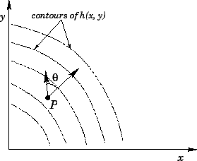 |
Consider a two-dimensional scalar field  , which is (say) the height of a hill.
Let
, which is (say) the height of a hill.
Let
 be an element of horizontal distance. Consider
 , where
  is the change in height after moving an infinitesimal distance
 . This quantity is somewhat like the one-dimensional gradient, except that
depends on the direction of , as well as its magnitude.
In the immediate vicinity of some point
. This quantity is somewhat like the one-dimensional gradient, except that
depends on the direction of , as well as its magnitude.
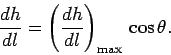
In the immediate vicinity of some point  , the slope reduces to an inclined plane (see Fig. 16).
The largest value of is straight up the slope. For any other direction
, the slope reduces to an inclined plane (see Fig. 16).
The largest value of is straight up the slope. For any other direction
 |
(93) |
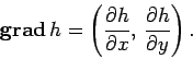
Let us define a two-dimensional vector,  ,
called the gradient of
,
called the gradient of  , whose magnitude is
 , and whose direction is the direction up the steepest slope.
Because of the
, and whose direction is the direction up the steepest slope.
Because of the  property, the component of in any
direction equals for that direction. [The argument, here, is analogous to
that used for vector areas in Sect. 2.3. See, in particular, Eq. (13).]
property, the component of in any
direction equals for that direction. [The argument, here, is analogous to
that used for vector areas in Sect. 2.3. See, in particular, Eq. (13).]
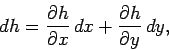
The component of in the -direction can be obtained by plotting out the
profile of at constant  , and then finding the slope of the tangent to the
curve at given . This quantity is known as the partial derivative of
with respect to at constant , and is denoted
, and then finding the slope of the tangent to the
curve at given . This quantity is known as the partial derivative of
with respect to at constant , and is denoted
 .
Likewise, the gradient of the profile at constant is written
.
Likewise, the gradient of the profile at constant is written
 . Note that the subscripts denoting constant- and
constant- are usually omitted, unless there is any ambiguity. If follows that
in component form
. Note that the subscripts denoting constant- and
constant- are usually omitted, unless there is any ambiguity. If follows that
in component form
 |
(94) |
Now, the equation of the tangent plane at
 is
is
 |
(95) |
This has the same local gradients as , so
 |
(96) |
by differentiation of the above.
For small  and
and  , the function is coincident with the tangent
plane. We have
, the function is coincident with the tangent
plane. We have
 |
(97) |
but
 and
, so
and
, so
 |
(98) |
Incidentally, the above equation demonstrates that is a proper vector,
since the left-hand side is a scalar, and, according to the properties of the dot
product, the right-hand side is also a scalar, provided that and
are both
proper vectors ( is an obvious vector, because it is
directly derived from displacements).
Consider, now, a three-dimensional temperature distribution  in
(say) a
reaction vessel. Let us define
in
(say) a
reaction vessel. Let us define
 , as before, as a vector whose magnitude is
 ,
and whose direction is the direction of the maximum gradient.
This vector is written in component form
,
and whose direction is the direction of the maximum gradient.
This vector is written in component form
 |
(99) |
Here,
 is the
gradient of the one-dimensional temperature profile at constant and
is the
gradient of the one-dimensional temperature profile at constant and  .
The change in
.
The change in  in going from point to a neighbouring point offset by
 is
is
 |
(100) |
In vector form, this becomes
 |
(101) |
Suppose that  for some . It follows that
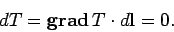 |
(102) |
So, is perpendicular to . Since along so-called
``isotherms'' (i.e., contours of the temperature), we conclude that the isotherms
(contours) are everywhere perpendicular to (see Fig. 17).
Figure 17:
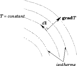 |
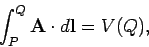
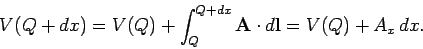
It is, of course, possible to integrate  . The line integral from point to
point
. The line integral from point to
point  is written
 |
(103) |
This integral is clearly independent of the path taken between and , so
 must be path independent.
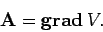
In general,
 depends on path,
but for some special vector fields the integral is path independent. Such fields
are called conservative fields. It can be shown that if
depends on path,
but for some special vector fields the integral is path independent. Such fields
are called conservative fields. It can be shown that if  is a
conservative field then
is a
conservative field then
 for some scalar field
  .
The proof of this is straightforward. Keeping fixed we have
.
The proof of this is straightforward. Keeping fixed we have
 |
(104) |
where  is a well-defined function, due to the path independent nature of the
line integral. Consider moving the position of the end point by an infinitesimal
amount
is a well-defined function, due to the path independent nature of the
line integral. Consider moving the position of the end point by an infinitesimal
amount  in the -direction. We have
 |
(105) |
Hence,
 |
(106) |
with analogous relations for the other components of . It follows that
 |
(107) |
In physics, the force due to gravity is a good example of a conservative field.
If is a force, then
 is the work done
in traversing some path. If is conservative then
is the work done
in traversing some path. If is conservative then
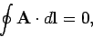 |
(108) |
where  corresponds to the line integral around some closed loop.
The fact that zero net work is done in going around a closed loop is equivalent
to the conservation of energy (this is why conservative fields are called
``conservative''). A good example of a non-conservative field is the force due
to friction. Clearly, a frictional system loses energy in going around a closed
cycle, so
corresponds to the line integral around some closed loop.
The fact that zero net work is done in going around a closed loop is equivalent
to the conservation of energy (this is why conservative fields are called
``conservative''). A good example of a non-conservative field is the force due
to friction. Clearly, a frictional system loses energy in going around a closed
cycle, so
 .
.
It is useful to define the vector operator
 |
(109) |
which is usually called the grad or del operator.
This operator acts on everything to
its right in a expression, until the end of the expression
or a closing bracket is reached.
For instance,
 |
(110) |
For two scalar fields and  ,
,
 |
(111) |
can be written more succinctly as
 |
(112) |
Suppose that we rotate the basis about the -axis by  degrees.
By analogy with Eqs. (7)-(9), the old coordinates (, , ) are related
to the new ones (
degrees.
By analogy with Eqs. (7)-(9), the old coordinates (, , ) are related
to the new ones ( ,
,  ,
,  ) via
) via
Now,
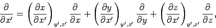 |
(116) |
giving
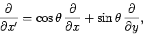 |
(117) |
and
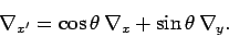 |
(118) |
It can be seen that
the differential operator  transforms like a proper vector,
according to Eqs. (10)-(12). This is another proof that
transforms like a proper vector,
according to Eqs. (10)-(12). This is another proof that  is a good vector.
Next: Divergence
Up: Vectors
Previous: Volume integrals
Richard Fitzpatrick
2006-02-02