 |
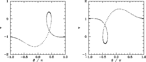 |
The interval
between the first and second chaotic regions is occupied by the period-1 orbits shown in
Figure 93. Note that these orbits differ somewhat from previously encountered period-1 orbits
in that the pendulum executes a complete rotation (either to
the left or to the right) every period of the external drive.
Now, an ![]() periodic orbit is defined such that
periodic orbit is defined such that
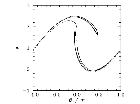 |
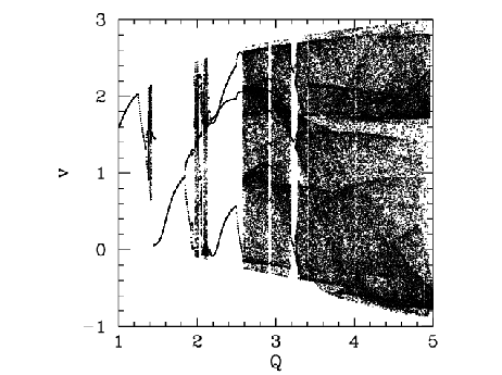
Figure 94 shows the Poincaré section of a typical attractor in the second chaotic region shown in Figure 92. It can be seen that this attractor is far more convoluted and extensive than the simple 4-line chaotic attractor pictured in Figure 82. In fact, the attractor shown in Figure 94 is clearly a fractal curve. It turns out that virtually all chaotic attractors exhibit fractal structure.
The interval between the second and third chaotic regions shown in Figure 92 is
occupied by ![]() ,
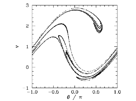
, ![]() periodic orbits. Figure 95 shows the Poincaré section
of a typical attractor in the
third chaotic region. It can be seen that this attractor is even more overtly fractal
in nature than that pictured in the previous figure. Note that the fractal nature
of chaotic attractors is closely associated with some of their unusual properties.
Trajectories on a chaotic attractor remain confined to a bounded region of phase-space,
and yet they separate from their neighbours exponentially fast (at least, initially).
How can trajectories diverge endlessly and still stay bounded? The basic mechanism
is described below.
If we imagine
a blob of initial conditions in phase-space then these undergo a series of
repeated stretching and folding episodes, as the chaotic motion unfolds. The stretching is
what gives rise to the divergence of neighbouring trajectories. The folding is what ensures that
the trajectories remain bounded.
The net
result is a phase-space structure which looks a bit like filo pastry--in other words, a fractal
structure.
periodic orbits. Figure 95 shows the Poincaré section
of a typical attractor in the
third chaotic region. It can be seen that this attractor is even more overtly fractal
in nature than that pictured in the previous figure. Note that the fractal nature
of chaotic attractors is closely associated with some of their unusual properties.
Trajectories on a chaotic attractor remain confined to a bounded region of phase-space,
and yet they separate from their neighbours exponentially fast (at least, initially).
How can trajectories diverge endlessly and still stay bounded? The basic mechanism
is described below.
If we imagine
a blob of initial conditions in phase-space then these undergo a series of
repeated stretching and folding episodes, as the chaotic motion unfolds. The stretching is
what gives rise to the divergence of neighbouring trajectories. The folding is what ensures that
the trajectories remain bounded.
The net
result is a phase-space structure which looks a bit like filo pastry--in other words, a fractal
structure.
 |