


Next: Sensitivity to Initial Conditions
Up: The Chaotic Pendulum
Previous: Period-Doubling Bifurcations
Route to Chaos
Let us return to Figure 73, which tracks the evolution of a left-favouring
periodic attractor as the quality-factor  is gradually increased. Recall that when
exceeds a critical value, which is about
is gradually increased. Recall that when
exceeds a critical value, which is about  , then the attractor
undergoes a period-doubling bifurcation which converts it from a period-1 to a period-2
attractor. This bifurcation is indicated by the forking of the curve in
Figure 73. Let us now investigate what happens as we continue to increase . Figure 77 is basically
a continuation of Figure 73. It can be seen that, as is gradually
increased, the attractor undergoes a period-doubling bifurcation at
, then the attractor
undergoes a period-doubling bifurcation which converts it from a period-1 to a period-2
attractor. This bifurcation is indicated by the forking of the curve in
Figure 73. Let us now investigate what happens as we continue to increase . Figure 77 is basically
a continuation of Figure 73. It can be seen that, as is gradually
increased, the attractor undergoes a period-doubling bifurcation at  , as before,
but then undergoes a second period-doubling bifurcation (indicated by the
second forking of
the curves) at
, as before,
but then undergoes a second period-doubling bifurcation (indicated by the
second forking of
the curves) at  , and a third bifurcation at
  . Obviously, the second bifurcation
converts a period-2 attractor into a period-4 attractor (hence, two curves split apart to
give four curves). Likewise, the third bifurcation converts a period-4 attractor
into a period-8 attractor (hence, four curves split into eight curves).
Shortly after the third
bifurcation, the various curves in the figure seem to expand explosively and merge together
to produce an area of almost solid black. As we shall see, this behaviour is indicative
of the onset of chaos.
. Obviously, the second bifurcation
converts a period-2 attractor into a period-4 attractor (hence, two curves split apart to
give four curves). Likewise, the third bifurcation converts a period-4 attractor
into a period-8 attractor (hence, four curves split into eight curves).
Shortly after the third
bifurcation, the various curves in the figure seem to expand explosively and merge together
to produce an area of almost solid black. As we shall see, this behaviour is indicative
of the onset of chaos.
Figure 77:
The  -coordinate of the Poincaré section of a time-asymptotic orbit
plotted against the quality-factor . Data
calculated numerically for
-coordinate of the Poincaré section of a time-asymptotic orbit
plotted against the quality-factor . Data
calculated numerically for
 ,
,  ,
,  ,
,  , and
, and  .
.
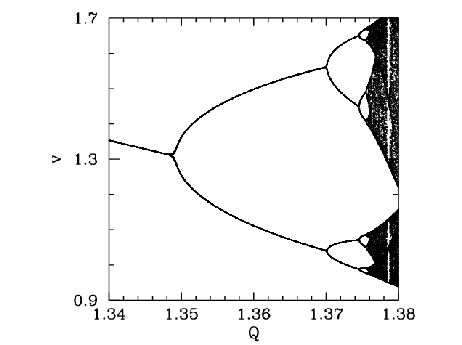 |
Figure 78 is a blow-up of Figure 77, showing more details of the onset of
chaos. The period-4 to period-8 bifurcation can be seen quite clearly. However,
we can also see a period-8 to period-16 bifurcation, at
 . Finally,
if we look carefully, we can see a hint of a period-16 to period-32 bifurcation, just
before the start of the solid black region.
Figures 77 and 78 seem to suggest that the
onset of chaos is triggered by an infinite series of period-doubling bifurcations.
. Finally,
if we look carefully, we can see a hint of a period-16 to period-32 bifurcation, just
before the start of the solid black region.
Figures 77 and 78 seem to suggest that the
onset of chaos is triggered by an infinite series of period-doubling bifurcations.
Figure 78:
The -coordinate of the Poincaré section of a time-asymptotic orbit
plotted against the quality-factor . Data
calculated numerically for
, , , ,
and .
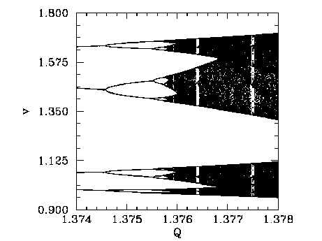 |
Table 5 gives some details of the sequence of period-doubling bifurcations
shown in Figures 77 and 78. Let us introduce a bifurcation index  : the
period-1 to period-2 bifurcation corresponds to
: the
period-1 to period-2 bifurcation corresponds to  ; the
period-2 to period-4 bifurcation corresponds to
; the
period-2 to period-4 bifurcation corresponds to  ; and so on. Let
  be
the critical value of the quality-factor at which the th bifurcation is
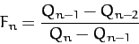
triggered. Table 5 shows the , determined from Figures 77 and 78, for
to 5. Also shown is the ratio
be
the critical value of the quality-factor at which the th bifurcation is
triggered. Table 5 shows the , determined from Figures 77 and 78, for
to 5. Also shown is the ratio
 |
(1251) |
for  to 5. It can be seen that Table 5 offers reasonably
convincing evidence that this ratio takes the constant value
to 5. It can be seen that Table 5 offers reasonably
convincing evidence that this ratio takes the constant value  .
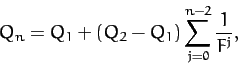
It follows that we can estimate the critical -value required to trigger the th
bifurcation via the following formula:
.
It follows that we can estimate the critical -value required to trigger the th
bifurcation via the following formula:
 |
(1252) |
for  . Note that the distance (in ) between bifurcations decreases rapidly as
increases. In fact, the above
formula predicts an accumulation of period-doubling bifurcations at
. Note that the distance (in ) between bifurcations decreases rapidly as
increases. In fact, the above
formula predicts an accumulation of period-doubling bifurcations at  , where
 |
(1253) |
Note that our calculated accumulation point corresponds almost exactly to the onset of the
solid black region in Figure 78.
By the time that exceeds  , we expect the attractor to have been
converted into a period-infinity
attractor via an infinite series of period-doubling bifurcations.
A period-infinity attractor is one whose corresponding motion never repeats
itself, no matter
how long we wait. In dynamics, such bounded aperiodic motion is generally referred to as chaos.
Hence, a period-infinity attractor is sometimes called a chaotic attractor.
Now, period- motion is represented by separate curves in Figure 78.
It is, therefore, not surprising that chaos (i.e., period-infinity motion) is
represented by an infinite number of curves which merge together to form a region of solid black.
, we expect the attractor to have been
converted into a period-infinity
attractor via an infinite series of period-doubling bifurcations.
A period-infinity attractor is one whose corresponding motion never repeats
itself, no matter
how long we wait. In dynamics, such bounded aperiodic motion is generally referred to as chaos.
Hence, a period-infinity attractor is sometimes called a chaotic attractor.
Now, period- motion is represented by separate curves in Figure 78.
It is, therefore, not surprising that chaos (i.e., period-infinity motion) is
represented by an infinite number of curves which merge together to form a region of solid black.
Table 5:
The period-doubling cascade.
| Bifurcation |
|
|
 |
 |
period-1 period-2 period-2 |
 |
 |
- |
- |
| period-2period-4 |
 |
 |
0.02133 |
- |
| period-4period-8 |
 |
 |
0.00455 |
 |
| period-8period-16 |
 |
 |
0.00097 |
 |
| period-16period-32 |
 |
 |
0.00020 |
 |
|
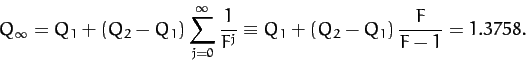
Let us examine the onset of chaos in a little more detail. Figures 79-82
show details of the pendulum's time-asymptotic motion at various stages on the
period-doubling cascade discussed above. Figure 79 shows period-4 motion:
note that the Poincaré section consists of four points, and the associated sequence of
net rotations per period of the pendulum repeats itself every four periods.
Figure 80 shows period-8 motion:
now the Poincaré section consists of eight points, and the rotation sequence
repeats itself every eight periods. Figure 81 shows period-16 motion:
as expected, the Poincaré section consists of sixteen points, and the rotation sequence
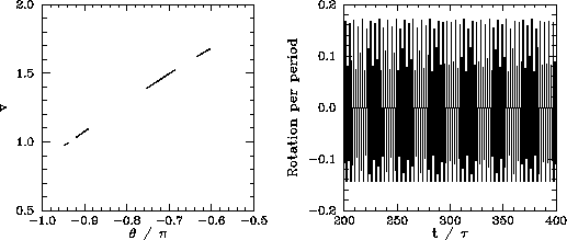
repeats itself every sixteen periods. Finally, Figure 82 shows chaotic motion. Note that
the Poincaré section now consists of a set of four continuous line segments, which are, presumably, made
up of an infinite number of points (corresponding to the infinite period of chaotic motion).
Note, also, that the associated sequence of net rotations per period shows no obvious sign of ever
repeating itself. In fact, this sequence looks rather like one of the previously shown periodic
sequences with the addition of a small random component. The generation of apparently
random motion from equations of motion, such as Equations (1237) and
(1238), which contain no overtly random elements is one of the most surprising features of
non-linear dynamics.
Figure 79:
The Poincaré section of a time-asymptotic orbit. Data
calculated numerically for  , , ,
, , and . Also, shown is the
net rotation per period,
, , ,
, , and . Also, shown is the
net rotation per period,
 , calculated at the Poincaré phase
.
, calculated at the Poincaré phase
.
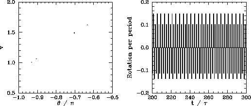 |
Figure 80:
The Poincaré section of a time-asymptotic orbit.
Data calculated numerically for  , , ,
, , and . Also, shown is the
net rotation per period,
, calculated at the Poincaré phase
.
, , ,
, , and . Also, shown is the
net rotation per period,
, calculated at the Poincaré phase
.
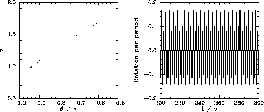 |
Figure 81:
The Poincaré section of a time-asymptotic orbit. Data
calculated numerically for  , , ,
, , and . Also, shown is the
net rotation per period,
, calculated at the Poincaré phase
.
, , ,
, , and . Also, shown is the
net rotation per period,
, calculated at the Poincaré phase
.
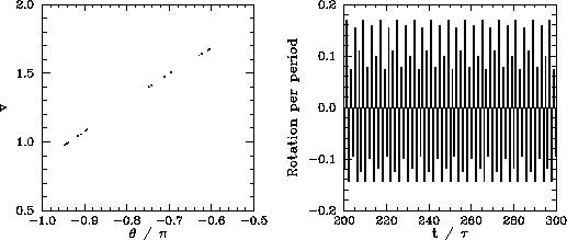 |
Figure 82:
The Poincaré section of a time-asymptotic orbit. Data
calculated numerically for  , , ,
, , and . Also, shown is the
net rotation per period,
, calculated at the Poincaré phase
.
, , ,
, , and . Also, shown is the
net rotation per period,
, calculated at the Poincaré phase
.
 |
Many non-linear dynamical systems found in nature exhibit a transition
from periodic to chaotic motion as some control parameter is varied.
Moreover, there are various known mechanisms by which chaotic motion can arise from periodic
motion. A transition to chaos via an infinite series of period-doubling bifurcations, as
illustrated
above, is one of the most commonly occurring mechanisms.
Around 1975, the physicist Mitchell Feigenbaum was investigating a simple mathematical
model, known as the logistic map, which exhibits a transition to chaos,
via a sequence of period-doubling bifurcations, as a control parameter
 is increased. Let
  be the value of at which the
first
be the value of at which the
first  -period cycle appears. Feigenbaum noticed that the ratio
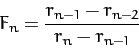 |
(1254) |
converges rapidly to a constant value,  , as increases. Feigenbaum was
able to demonstrate that this value of
, as increases. Feigenbaum was
able to demonstrate that this value of  is common to a wide range of different
mathematic models which exhibit transitions to chaos via period-doubling
bifurcations.
is common to a wide range of different
mathematic models which exhibit transitions to chaos via period-doubling
bifurcations.![[*]](footnote.png) Feigenbaum went on to argue that the Feigenbaum ratio, ,
should converge to the value
Feigenbaum went on to argue that the Feigenbaum ratio, ,
should converge to the value  in any dynamical system exhibiting a
transition to chaos via period-doubling bifurcations. This amazing prediction has
been verified experimentally in a number of quite different physical
systems. Note that our best estimate of the
Feigenbaum ratio (see Table 5) is , in good agreement with Feigenbaum's
prediction.
in any dynamical system exhibiting a
transition to chaos via period-doubling bifurcations. This amazing prediction has
been verified experimentally in a number of quite different physical
systems. Note that our best estimate of the
Feigenbaum ratio (see Table 5) is , in good agreement with Feigenbaum's
prediction.
The existence of a universal ratio characterizing the transition to chaos via
period-doubling bifurcations is one of many pieces of evidence indicating that
chaos is a universal phenomenon (i.e., the onset and nature
of chaotic motion in different dynamical systems has many common features).
This observation encourages us to believe that in studying the chaotic motion of
a damped periodically driven pendulum we are learning lessons which can
be applied to a wide range of non-linear dynamical systems.
Next: Sensitivity to Initial Conditions
Up: The Chaotic Pendulum
Previous: Period-Doubling Bifurcations
Richard Fitzpatrick
2011-03-31