 |
Let us return to Figure 78. Recall, that this figure shows the onset of
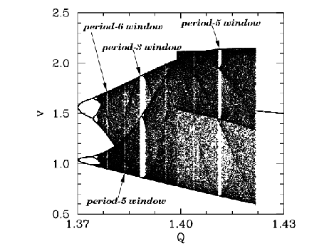
chaos, via a cascade of period-doubling bifurcations, as the quality-factor ![]() is gradually increased. Figure 87 is essentially a continuation of Figure 78
which shows the full extent of the chaotic region (in
is gradually increased. Figure 87 is essentially a continuation of Figure 78
which shows the full extent of the chaotic region (in ![]() -
-![]() space). It can be
seen that the chaotic region ends abruptly when
space). It can be
seen that the chaotic region ends abruptly when ![]() exceeds a critical
value, which is about
exceeds a critical
value, which is about ![]() . Beyond this critical value, the time-asymptotic motion appears to
revert to period-1 motion (i.e., the solid black region collapses to a single curve).
It can also be seen that the chaotic region contains many narrow windows in which
chaos reverts to periodic motion (i.e., the solid black region collapses
to
. Beyond this critical value, the time-asymptotic motion appears to
revert to period-1 motion (i.e., the solid black region collapses to a single curve).
It can also be seen that the chaotic region contains many narrow windows in which
chaos reverts to periodic motion (i.e., the solid black region collapses
to ![]() curves, where
curves, where ![]() is the period of the motion) for a short interval in
is the period of the motion) for a short interval in ![]() . The four widest
windows are indicated in the figure.
. The four widest
windows are indicated in the figure.
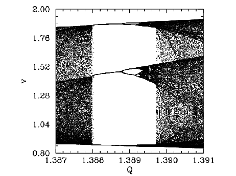 |
Figure 88 is a blow-up of the period-3 window shown in Figure 87. It can be
seen that the window appears ``out of the blue'' as ![]() is gradually increased. However,
it can also be seen that, as
is gradually increased. However,
it can also be seen that, as ![]() is further increased, the window breaks down,
and eventually disappears, due to the action of a cascade of period-doubling
bifurcations. The same basic mechanism operates here as in the original period-doubling
cascade, discussed in Section 15.9, except that now the orbits are of period
is further increased, the window breaks down,
and eventually disappears, due to the action of a cascade of period-doubling
bifurcations. The same basic mechanism operates here as in the original period-doubling
cascade, discussed in Section 15.9, except that now the orbits are of period ![]() , instead of
, instead of ![]() .
Note that all of the other periodic windows seen in Figure 87 break down in an analogous manner,
as
.
Note that all of the other periodic windows seen in Figure 87 break down in an analogous manner,
as ![]() is increased.
is increased.
 |
 |
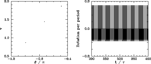 |
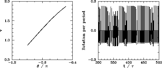
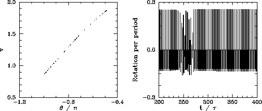
We now understand how periodic windows break down. But, how do they appear in the first place? Figures 89-91 show details of the pendulum's time-asymptotic motion calculated just before the appearance of the period-3 window (shown in Figure 88), just at the appearance of the window, and just after the appearance of the window, respectively. It can be seen, from Figure 89, that just before the appearance of the window the attractor is chaotic (i.e., its Poincaré section consists of a line, rather than a discrete set of points), and the time-asymptotic motion of the pendulum consists of intervals of period-3 motion interspersed with intervals of chaotic motion. Figure 90 shows that just at the appearance of the window the attractor loses much of its chaotic nature (i.e., its Poincaré section breaks up into a series of points), and the chaotic intervals become shorter and much less frequent. Finally, Figure 91 shows that just after the appearance of the window the attractor collapses to a period-3 attractor, and the chaotic intervals cease altogether. All of the other periodic windows seen in Figure 87 appear in an analogous manner to that just described.
According to the above discussion,
the typical time-asymptotic motion seen just prior to the appearance of a period-![]() window
consists of intervals of period-
window
consists of intervals of period-![]() motion interspersed with intervals of chaotic
motion. This type of behaviour is called intermittency, and is observed in a
wide variety of non-linear systems. As we move away from the window, in parameter
space, the intervals of periodic motion become gradually shorter and more infrequent.
Eventually, they cease altogether. Likewise, as we move towards the window, the
intervals of periodic motion become gradually longer and more frequent. Eventually,
the whole motion becomes periodic.
motion interspersed with intervals of chaotic
motion. This type of behaviour is called intermittency, and is observed in a
wide variety of non-linear systems. As we move away from the window, in parameter
space, the intervals of periodic motion become gradually shorter and more infrequent.
Eventually, they cease altogether. Likewise, as we move towards the window, the
intervals of periodic motion become gradually longer and more frequent. Eventually,
the whole motion becomes periodic.
In 1973, Metropolis and co-workers investigated a class of simple mathematical models which all
exhibit a transition to chaos, via a cascade of period-doubling bifurcations, as
some control parameter ![]() is increased.
is increased.![[*]](footnote.png) They were able to demonstrate
that, for these models, the order in which stable periodic orbits occur as
They were able to demonstrate
that, for these models, the order in which stable periodic orbits occur as ![]() is
increased is fixed.
That is, stable periodic attractors always occur in the same sequence as
is
increased is fixed.
That is, stable periodic attractors always occur in the same sequence as
![]() is varied. This sequence is
called the universal or U-sequence. It is possible to make a fairly
convincing argument that any physical system which exhibits a transition to chaos
via a sequence of period-doubling bifurcations should also exhibit the U-sequence
of stable periodic attractors.
Up to period-6, the U-sequence is
is varied. This sequence is
called the universal or U-sequence. It is possible to make a fairly
convincing argument that any physical system which exhibits a transition to chaos
via a sequence of period-doubling bifurcations should also exhibit the U-sequence
of stable periodic attractors.
Up to period-6, the U-sequence is
The existence of
a universal sequence of stable periodic orbits in dynamical systems which
exhibit a transition to chaos via a cascade of period-doubling bifurcations
is another indication that
chaos is a universal phenomenon.