Next: Two-Dimensional Vortex Filaments
Up: Two-Dimensional Incompressible Inviscid Flow
Previous: Two-Dimensional Uniform Flow
Two-Dimensional Sources and Sinks
Consider a uniform line source, coincident with the  -axis,
that emits fluid isotropically at the steady rate of
-axis,
that emits fluid isotropically at the steady rate of  unit volumes per unit length per unit time.
By symmetry, we expect the associated steady flow pattern to be isotropic, and everywhere directed radially away from the source.
(See Figure 5.3.) In other words, we expect
unit volumes per unit length per unit time.
By symmetry, we expect the associated steady flow pattern to be isotropic, and everywhere directed radially away from the source.
(See Figure 5.3.) In other words, we expect
 |
(5.31) |
where
 .
Consider a cylindrical surface
.
Consider a cylindrical surface  of unit height (in the
-direction) and radius
of unit height (in the
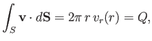
-direction) and radius  that is co-axial with the source. In a steady state,
the rate at which fluid crosses this surface must be equal to the rate at which the
section of the source enclosed by the surface emits fluid. Hence,
that is co-axial with the source. In a steady state,
the rate at which fluid crosses this surface must be equal to the rate at which the
section of the source enclosed by the surface emits fluid. Hence,
 |
(5.32) |
which implies that
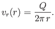 |
(5.33) |
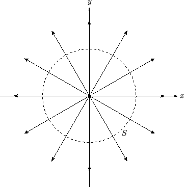
Figure:
Streamlines of the flow generated by a line source coincident with the
-axis.
 |
According to Equations (5.13) and (5.14), the stream function associated with a line source
of strength
that is coincident with the
-axis is
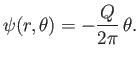 |
(5.34) |
Note that the streamlines,  , are directed radially away from the
-axis, as illustrated in Figure 5.3.
Note, also, that the stream function associated with a line source is multivalued. However, this does not cause any
particular difficulty,
because the stream function is continuous, and its gradient is single valued.
, are directed radially away from the
-axis, as illustrated in Figure 5.3.
Note, also, that the stream function associated with a line source is multivalued. However, this does not cause any
particular difficulty,
because the stream function is continuous, and its gradient is single valued.
It follows from Equation (5.34) that
 . Hence,
according to Equation (5.15),
. Hence,
according to Equation (5.15),
 . In other words, the steady flow pattern
associated with a uniform line source is irrotational, and can, thus, be derived from a velocity
potential. In fact, it is easily demonstrated that this potential takes the form
. In other words, the steady flow pattern
associated with a uniform line source is irrotational, and can, thus, be derived from a velocity
potential. In fact, it is easily demonstrated that this potential takes the form
 |
(5.35) |
A uniform line sink, coincident with the
-axis,
which absorbs fluid isotropically at the steady rate of
unit volumes per unit length per unit time
has an associated steady flow pattern
 |
(5.36) |
whose stream function is
 |
(5.37) |
This flow pattern is also irrotational, and can be derived from the velocity potential
 |
(5.38) |
Consider a line source and a line sink of equal strength, which both run parallel to the
-axis, and are located a small distance apart in the  -
- plane. Such an arrangement
is known as a doublet or dipole line source. Suppose that the line source, which is of strength
, is located
at
plane. Such an arrangement
is known as a doublet or dipole line source. Suppose that the line source, which is of strength
, is located
at
 (where
  is a position vector in the
-
plane), and that the line sink, which is also of strength
, is located at
is a position vector in the
-
plane), and that the line sink, which is also of strength
, is located at
 .
Let the function
.
Let the function
 |
(5.39) |
be the stream function associated with a line source of strength
located at
 .
Thus,
.
Thus,
 is the stream function associated with a line source of strength
located at
is the stream function associated with a line source of strength
located at
 .
Furthermore, the stream function associated with a line sink of strength
located at
is
.
Furthermore, the stream function associated with a line sink of strength
located at
is
 . We expect the flow pattern associated with the combination of a source and a sink to be the vector
sum of the flow patterns generated by the source and sink taken in isolation. It follows that the overall stream function
is the sum of the stream functions generated by the source and the sink taken in isolation. In other words,
. We expect the flow pattern associated with the combination of a source and a sink to be the vector
sum of the flow patterns generated by the source and sink taken in isolation. It follows that the overall stream function
is the sum of the stream functions generated by the source and the sink taken in isolation. In other words,
 |
(5.40) |
to first order in  . Hence, if
![$ {\bf d} = d\,(\cos\theta_0\,{\bf e}_x+ \sin\theta_0\,{\bf e}_y)=d\,[\cos(\theta-\theta_0)\,{\bf e}_r
-\sin(\theta-\theta_0)\,{\bf e}_\theta]$](img1690.png) ,
so that the line joining the sink to the source subtends a (counter-clockwise) angle
,
so that the line joining the sink to the source subtends a (counter-clockwise) angle  with the
-axis,
then
with the
-axis,
then
 |
(5.41) |
where  is termed the strength of the dipole source. The previous stream function is antisymmetric
across the line
is termed the strength of the dipole source. The previous stream function is antisymmetric
across the line
 joining the source to the sink. It follows that the
associated dipole flow pattern,
joining the source to the sink. It follows that the
associated dipole flow pattern,
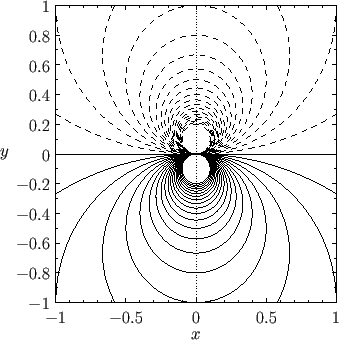
is symmetric across this line. Figure 5.4 shows the streamlines associated with a dipole flow
pattern characterized by  and
and
 . Note that the flow speed in a dipole
pattern falls off like
. Note that the flow speed in a dipole
pattern falls off like  .
.
Figure:
Streamlines of the flow generated by a dipole line source (with
) coincident with the
-axis, and
aligned along the
-axis. The flow is outward along the positive
-axis and inward
along the negative
-axis. Positive and negative contours are shown as solid and dashed lines,
respectively.
 |
A dipole flow pattern is necessarily irrotational because it is a linear superposition of two irrotational flow patterns.
The associated velocity potential is
 |
(5.44) |
Next: Two-Dimensional Vortex Filaments
Up: Two-Dimensional Incompressible Inviscid Flow
Previous: Two-Dimensional Uniform Flow
Richard Fitzpatrick
2016-03-31