Next: Circulation and Vorticity
Up: Incompressible Inviscid Flow
Previous: Flow over a Broad-Crested
The curl of the velocity field of a fluid, which is generally termed vorticity, is usually
represented by the symbol
 , so that
  |
(4.71) |
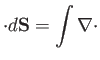
A vortex line is a line whose tangent is everywhere parallel to the local vorticity vector.
The vortex lines drawn through each point of a closed curve
constitute the surface of a vortex tube. Finally, a
vortex filament is a vortex tube whose cross-section is of infinitesimal dimensions.
Figure 4.9:
A vortex filament.
 |
Consider a section  of a vortex filament. The filament is bounded by the curved surface that forms the filament
wall, as well as two plane surfaces, whose vector areas are
of a vortex filament. The filament is bounded by the curved surface that forms the filament
wall, as well as two plane surfaces, whose vector areas are  and
and  (say), which form the ends of the section at
points
(say), which form the ends of the section at
points  and
and  , respectively. (See Figure 4.9.) Let the plane surfaces have outward pointing normals
that are parallel (or anti-parallel) to the vorticity vectors,
, respectively. (See Figure 4.9.) Let the plane surfaces have outward pointing normals
that are parallel (or anti-parallel) to the vorticity vectors,
 and
and
 , at points
and
,
respectively.
The divergence theorem (see Section A.20), applied to the section, yields
, at points
and
,
respectively.
The divergence theorem (see Section A.20), applied to the section, yields
where  is an outward directed surface element, and
  a volume element. However,
[see Equation (A.173)],
implying that
Now,
 on the curved surface of the filament,
because
is, by definition, tangential to this surface. Thus, the only contributions to the surface integral
come from the plane areas
and
. It follows that
on the curved surface of the filament,
because
is, by definition, tangential to this surface. Thus, the only contributions to the surface integral
come from the plane areas
and
. It follows that
This result is essentially an equation of continuity for vortex filaments. It implies that the product of the
magnitude of the vorticity and the cross-sectional area, which is termed the vortex intensity, is constant
along the filament. It follows that a vortex filament cannot terminate in the interior of the fluid. For, if
it did, the cross-sectional area,  , would have to vanish, and, therefore, the vorticity,
, would have to become infinite. Thus,
a vortex filament must either form a closed vortex ring, or must terminate at the fluid boundary.
, would have to vanish, and, therefore, the vorticity,
, would have to become infinite. Thus,
a vortex filament must either form a closed vortex ring, or must terminate at the fluid boundary.
Because a vortex tube can be regarded as a bundle of vortex filaments whose net intensity is the sum of the
intensities of the constituent filaments, we conclude that the intensity of a vortex tube
remains constant along the tube.
Next: Circulation and Vorticity
Up: Incompressible Inviscid Flow
Previous: Flow over a Broad-Crested
Richard Fitzpatrick
2016-03-31