Maxwell-Boltzmann Statistics

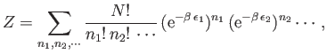
For the purpose of comparison, it is instructive to consider the purely classical case of Maxwell-Boltzmann statistics. The partition function is written

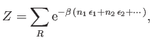$$Z=\sum_{R} {\rm e}^{-\beta (n_1 \epsilon_1+n_2 \epsilon_2+\cdots)},$$ (8.46)

where the sum is over all distinct states $R$ of the gas, and the particles are treated as distinguishable. For given values of $n_1, n_2,\cdots$ there are

$$\frac{N!}{n_1 ! n_2! \cdots}$$ (8.47)

possible ways in which $N$ distinguishable particles can be put into individual quantum states such that there are $n_1$ particles in state 1, $n_2$ particles in state 2, et cetera. Each of these possible arrangements corresponds to a distinct state for the whole gas. Hence, Equation (8.46) can be written

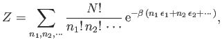$$Z = \sum_{n_1,n_2,\cdots} \frac{N!}{n_1 ! n_2! \cdots} {\rm e}^{-\beta (n_1 \epsilon_1+n_2 \epsilon_2+\cdots)},$$ (8.48)

where the sum is over all values of $n_r=0,1,2,\cdots$ for each $r$ , subject to the constraint that

$$\sum_r n_r = N.$$ (8.49)

Now, Equation (8.48) can be written

$$Z = \sum_{n_1,n_2,\cdots} \frac{N!}{n_1 ! n_2! \cdots} ({\rm e}^{-\beta \epsilon_1})^{n_1} ({\rm e}^{-\beta \epsilon_2})^{n_2} \cdots,$$ (8.50)

which, by virtue of Equation (8.49), is just the result of expanding a polynomial. In fact,

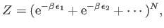$$Z = ({\rm e}^{-\beta \epsilon_1}+{\rm e}^{-\beta \epsilon_2}+ \cdots)^N,$$ (8.51)

or

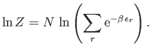$$\ln Z = N \ln\left(\sum_r {\rm e}^{-\beta \epsilon_r}\right).$$ (8.52)

Note that the argument of the logarithm is simply the single-particle partition function

Equations (8.20) and (8.52) can be combined to give

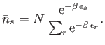$$\bar{n}_s = N \frac{{\rm e}^{-\beta \epsilon_s}} {\sum_r {\rm e}^{-\beta \epsilon_r}}.$$ (8.53)

This is known as the Maxwell-Boltzmann distribution. It is, of course, just the result obtained by applying the canonical distribution to a single particle. (See Chapter 7.) The previous expression can also be written in the form

$$\bar{n}_s = {\rm e}^{-\alpha-\beta \epsilon_r},$$ (8.54)

where

$$\sum_r {\rm e}^{-\alpha-\beta \epsilon_r} = N.$$ (8.55)

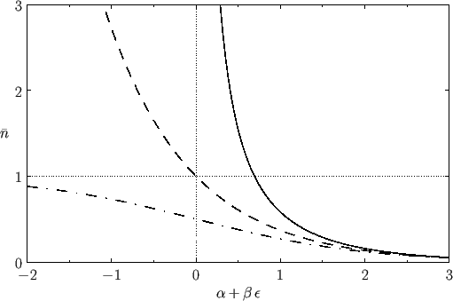
The Bose-Einstein, Maxwell-Boltzmann, and Fermi-Dirac distributions are illustrated in Figure 8.1.

Figure 8.1: A comparison of the Bose-Einstein (solid curve), Maxwell-Boltzmann (dashed curve), and Fermi-Dirac (dash-dotted curve) distributions.