Next: Two Spin One-Half Particles
Up: Addition of Angular Momentum
Previous: General Principles
Angular Momentum in the Hydrogen Atom
In a hydrogen atom, the wavefunction of an electron in a simultaneous
eigenstate of  and
and  has an angular dependence specified
by the spherical harmonic
has an angular dependence specified
by the spherical harmonic
 (see Sect. 8.7).
If the electron is also in an eigenstate of
(see Sect. 8.7).
If the electron is also in an eigenstate of  and
and  then the
quantum numbers
then the
quantum numbers  and
and  take the values
  and
and  ,
respectively, and the internal state of the electron is specified
by the spinors
,
respectively, and the internal state of the electron is specified
by the spinors  (see Sect. 10.5). Hence, the
simultaneous eigenstates of , , , and can be written
in the separable form
(see Sect. 10.5). Hence, the
simultaneous eigenstates of , , , and can be written
in the separable form
 |
(806) |
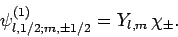
Here, it is understood that orbital angular momentum operators act on
the spherical harmonic functions,  , whereas spin angular momentum operators act
on the spinors, .
, whereas spin angular momentum operators act
on the spinors, .
Since the eigenstates
 are (presumably)
orthonormal, and form a complete set, we can express the eigenstates
are (presumably)
orthonormal, and form a complete set, we can express the eigenstates
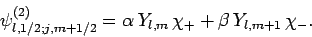
 as linear combinations of them. For instance,
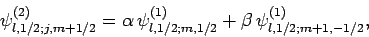 |
(807) |
where  and
and  are, as yet, unknown coefficients. Note that
the number of
are, as yet, unknown coefficients. Note that
the number of  states which can appear on the right-hand side
of the above expression is limited to two by the constraint that
states which can appear on the right-hand side
of the above expression is limited to two by the constraint that
 [see Eq. (801)], and the fact that can only take the values .
Assuming that the
[see Eq. (801)], and the fact that can only take the values .
Assuming that the  eigenstates are properly normalized, we have
 |
(808) |
Now, it follows from Eq. (804) that
 |
(809) |
where [see Eq. (790)]
 |
(810) |
Moreover, according to Eqs. (806) and (807), we can write
 |
(811) |
Recall, from Eqs. (568) and (569), that
By analogy, when the spin raising and lowering operators,  , act on a general spinor,
  , we obtain
For the special case of spin one-half spinors (i.e.,
 ), the above expressions reduce to
 |
(816) |
and
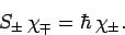 |
(817) |
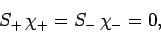
It follows from Eqs. (810) and (812)-(817) that
and
Hence, Eqs. (809) and (811) yield
where
 |
(822) |
Equations (820) and (821) can be solved to give
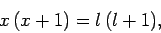 |
(823) |
and
![\begin{displaymath}
\frac{\alpha}{\beta} = \frac{[(l-m) (l+m+1)]^{1/2}}{x-m}.
\end{displaymath}](img1950.png) |
(824) |
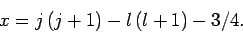
It follows that  or
or  , which corresponds to
  or
or
 , respectively. Once
  is specified, Eqs. (808) and (824) can be solved for and . We obtain
 |
(825) |
and
 |
(826) |
Here, we have neglected the common subscripts  for the sake of
clarity: i.e.,
for the sake of
clarity: i.e.,
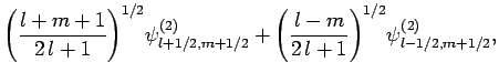
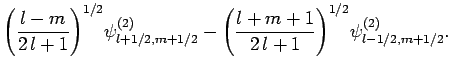
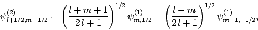
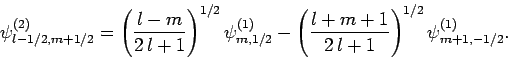
 , etc. The above equations can easily be inverted
to give the eigenstates in terms of the eigenstates:
, etc. The above equations can easily be inverted
to give the eigenstates in terms of the eigenstates:
The information contained in Eqs. (825)-(828)
is neatly summarized in Table 2. For instance, Eq. (825)
is obtained by reading the first row of this table, whereas Eq. (828)
is obtained by reading the second column. The coefficients in this type
of table are generally known as Clebsch-Gordon coefficients.
Table 2:
Clebsch-Gordon coefficients for adding spin one-half to
spin  .
.
|
|
As an example, let us consider the  states of a hydrogen atom.
The eigenstates of , , , and ,
are denoted
states of a hydrogen atom.
The eigenstates of , , , and ,
are denoted
 . Since
  can take the values
  ,
whereas can take the values , there are
clearly six such states: i.e.,
,
whereas can take the values , there are
clearly six such states: i.e.,
 ,
,
 ,
and
,
and
 . The eigenstates of , ,
  , and
, and  ,
are denoted
,
are denoted
 . Since and
  can be combined
together to form either
can be combined
together to form either  or
or  (see earlier), there are
also six such states: i.e.,
(see earlier), there are
also six such states: i.e.,
 ,
,
 , and
, and
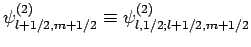
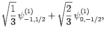
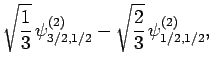
 . According to
Table 2, the various different eigenstates are interrelated as follows:
. According to
Table 2, the various different eigenstates are interrelated as follows:
 |
 |
 |
(829) |
 |
|
 |
(830) |
 |
|
 |
(831) |
 |
|
 |
(832) |
 |
|
 |
(833) |
and
 |
|
 |
(834) |
 |
|
 |
(835) |
 |
|
 |
(836) |
 |
|
 |
(837) |
 |
|
 |
(838) |
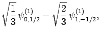
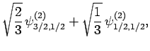
Thus, if we know that an electron in a hydrogen atom is in an
state characterized by  and
and  [i.e., the state
represented by
[i.e., the state
represented by
 ] then, according to Eq. (836),
a measurement of the total angular momentum will yield ,
] then, according to Eq. (836),
a measurement of the total angular momentum will yield ,  with probability
  , and , with probability
  .
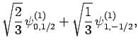
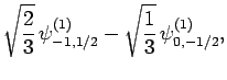
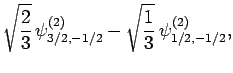
Suppose that we make such a measurement, and obtain the result , . As a result of the measurement, the electron is thrown into
the corresponding eigenstate,
.
Suppose that we make such a measurement, and obtain the result , . As a result of the measurement, the electron is thrown into
the corresponding eigenstate,
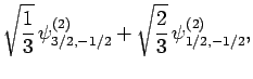
 . It thus follows
from Eq. (830) that a subsequent measurement of and
will yield , with probability , and
. It thus follows
from Eq. (830) that a subsequent measurement of and
will yield , with probability , and  ,
,  with probability .
Table 3:
Clebsch-Gordon coefficients for adding spin one-half to
spin one. Only non-zero coefficients are shown.
|
|
The information contained in Eqs. (829)-(837) is neatly summed
up in Table 3. Note that each row and column of this
table has unit norm, and also that the different rows and different columns
are mutually orthogonal. Of course, this is because the and
eigenstates are orthonormal.
Next: Two Spin One-Half Particles
Up: Addition of Angular Momentum
Previous: General Principles
Richard Fitzpatrick
2010-07-20