


Next: Exercises
Up: Orbital Angular Momentum
Previous: Eigenvalues of
Spherical Harmonics
The simultaneous eigenstates,
 , of
, of  and
and  are known as the spherical harmonics. Let us investigate their
functional form.
are known as the spherical harmonics. Let us investigate their
functional form.
Now, we know that
 |
(591) |
since there is no state for which  has a larger value than
  .
Writing
.
Writing
 |
(592) |
[see Eqs. (570) and (574)], and making use of
Eq. (555), we obtain
 |
(593) |
This equation yields
 |
(594) |
which can easily be solved to give
 |
(595) |
Hence, we conclude that
 |
(596) |
Likewise, it is easy to demonstrate that
 |
(597) |
Once we know  , we can obtain
  by operating
on with the lowering operator
by operating
on with the lowering operator  . Thus,
 |
(598) |
where use has been made of Eq. (555).
The above equation yields
 |
(599) |
Now,
![\begin{displaymath}
\left(\frac{d}{d\theta}+l \cot\theta\right)f(\theta)\equiv
...
...a)^l}\frac{d}{d\theta}\left[
(\sin\theta)^l f(\theta)\right],
\end{displaymath}](img1448.png) |
(600) |
where  is a general function. Hence, we can write
 |
(601) |
Likewise, we can show that
 |
(602) |
We can now obtain  by operating on with the
lowering operator. We get
by operating on with the
lowering operator. We get
 |
(603) |
which reduces to
 |
(604) |
Finally, making use of Eq. (600), we obtain
 |
(605) |
Likewise, we can show that
 |
(606) |
A comparison of Eqs. (596), (601), and (605)
reveals the general functional form of the spherical harmonics:
 |
(607) |
Here, is assumed to be non-negative. Making the substitution  , we can also write
 |
(608) |
Finally, it is clear from Eqs. (597), (602), and (606)
that
 |
(609) |
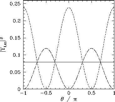
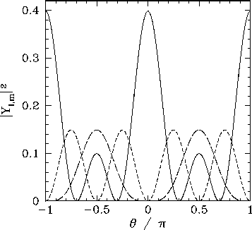
Figure 18:
The
 plotted as a functions of
  . The solid, short-dashed, and long-dashed curves correspond to
 , and
, and  , and
, and  , respectively.
 |
We now need to normalize our spherical harmonic functions so as to ensure that
 |
(610) |
After a great deal of tedious analysis, the normalized spherical
harmonic functions are found to take the form
![\begin{displaymath}
Y_{l,m}(\theta,\phi) =(-1)^m \left[\frac{2 l+1}{4\pi} \f...
...right]^{1/2} P_{l,m}(\cos\theta) {\rm e}^{ {\rm i} m \phi}
\end{displaymath}](img1463.png) |
(611) |
for  , where the
  are known as associated Legendre
polynomials, and are written
are known as associated Legendre
polynomials, and are written
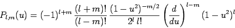 |
(612) |
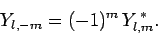
for . Alternatively,
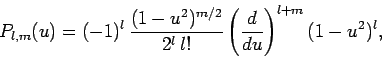 |
(613) |
for .
The spherical harmonics characterized by  can be calculated from those characterized by
  via the identity
 |
(614) |
The spherical harmonics are orthonormal: i.e.,
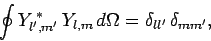 |
(615) |
and also form a complete set. In other words,
any function of and  can be represented as
a superposition of spherical harmonics. Finally, and most importantly,
the spherical harmonics are the simultaneous eigenstates of and
corresponding to the eigenvalues
can be represented as
a superposition of spherical harmonics. Finally, and most importantly,
the spherical harmonics are the simultaneous eigenstates of and
corresponding to the eigenvalues  and
and
 ,
respectively.
,
respectively.
Figure 19:
The
plotted as a functions of . The solid, short-dashed, and long-dashed curves correspond to
 , and
, and  , and
, and  , respectively.
 |
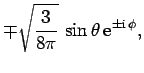
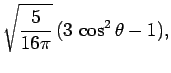
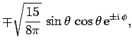
All of the  ,
,  , and
, and  spherical harmonics are listed below:
 |
 |
 |
(616) |
 |
|
 |
(617) |
 |
|
 |
(618) |
 |
|
 |
(619) |
 |
|
 |
(620) |
 |
|
 |
(621) |
The variation of these functions is illustrated in Figs. 18 and
19.
Subsections
Next: Exercises
Up: Orbital Angular Momentum
Previous: Eigenvalues of
Richard Fitzpatrick
2010-07-20