Wave Packets

The above discussion suggests that the wavefunction of a massive particle of momentum $p$ and energy $E$, moving in the positive $x$-direction, can be written

$$\psi(x,t) = \bar{\psi} {\rm e}^{ {\rm i} (k x-\omega t)},$$ (82)

where $k= p/\hbar>0$ and $\omega = E/\hbar>0$. Here, $\omega$ and $k$ are linked via the dispersion relation (79). Expression (82) represents a plane wave whose maxima and minima propagate in the positive $x$-direction with the phase velocity $v_p=\omega/k$. As we have seen, this phase velocity is only half of the classical velocity of a massive particle.

From before, the most reasonable physical interpretation of the wavefunction is that $\vert\psi(x,t)\vert^{ 2}$ is proportional to the probability density of finding the particle at position $x$ at time $t$. However, the modulus squared of the wavefunction (82) is $\vert\bar{\psi}\vert^{ 2}$, which depends on neither $x$ nor $t$. In other words, this wavefunction represents a particle which is equally likely to be found anywhere on the $x$-axis at all times. Hence, the fact that the maxima and minima of the wavefunction propagate at a phase velocity which does not correspond to the classical particle velocity does not have any real physical consequences.

So, how can we write the wavefunction of a particle which is localized in $x$: i.e., a particle which is more likely to be found at some positions on the $x$-axis than at others? It turns out that we can achieve this goal by forming a linear combination of plane waves of different wavenumbers: i.e.,

$$\psi(x,t) = \int_{-\infty}^{\infty} \bar{\psi}(k) {\rm e}^{ {\rm i} (k x-\omega t)} dk.$$ (83)

Here, $\bar{\psi}(k)$ represents the complex amplitude of plane waves of wavenumber $k$ in this combination. In writing the above expression, we are relying on the assumption that particle waves are superposable: i.e., it is possible to add two valid wave solutions to form a third valid wave solution. The ultimate justification for this assumption is that particle waves satisfy a differential wave equation which is linear in $\psi$. As we shall see, in Sect. 3.15, this is indeed the case. Incidentally, a plane wave which varies as $\exp[{\rm i} (k x-\omega t)]$ and has a negative $k$ (but positive $\omega$) propagates in the negative $x$-direction at the phase velocity $\omega/\vert k\vert$. Hence, the superposition (83) includes both forward and backward propagating waves.

Now, there is a useful mathematical theorem, known as Fourier's theorem, which states that if

$$f(x) = \frac{1}{\sqrt{2\pi}}\int_{-\infty}^{\infty} \bar{f}(k) {\rm e}^{ {\rm i} k x} dk,$$ (84)

then

$$\bar{f}(k) = \frac{1}{\sqrt{2\pi}}\int_{-\infty}^\infty f(x) {\rm e}^{-{\rm i} k x} dx.$$ (85)

Here, $\bar{f}(k)$ is known as the Fourier transform of the function $f(x)$. We can use Fourier's theorem to find the $k$-space function $\bar{\psi}(k)$ which generates any given $x$-space wavefunction $\psi(x)$ at a given time.

For instance, suppose that at $t=0$ the wavefunction of our particle takes the form

$$\psi(x,0) \propto \exp\left[{\rm i} k_0 x - \frac{(x-x_0)^{ 2}}{4 ({\mit\Delta}x)^{ 2}}\right].$$ (86)

Thus, the initial probability density of the particle is written

$$\vert\psi(x,0)\vert^{ 2} \propto \exp\left[- \frac{(x-x_0)^{ 2}}{2 ({\mit\Delta}x)^{ 2}}\right].$$ (87)

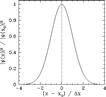
This particular probability distribution is called a Gaussian distribution, and is plotted in Fig. 7. It can be seen that a measurement of the particle's position is most likely to yield the value $x_0$, and very unlikely to yield a value which differs from $x_0$ by more than $3 {\mit\Delta} x$. Thus, (86) is the wavefunction of a particle which is initially localized around $x=x_0$ in some region whose width is of order ${\mit\Delta} x$. This type of wavefunction is known as a wave packet.

Figure 7: A Gaussian probability distribution in $x$-space.

Now, according to Eq. (83),

$$\psi(x,0) = \int_{-\infty}^{\infty} \bar{\psi}(k) {\rm e}^{ {\rm i} k x} dk.$$ (88)

Hence, we can employ Fourier's theorem to invert this expression to give

$$\bar{\psi}(k)\propto \int_{-\infty}^{\infty} \psi(x,0) {\rm e}^{-{\rm i} k x} dx.$$ (89)

Making use of Eq. (86), we obtain

$$\bar{\psi}(k) \propto {\rm e}^{-{\rm i} (k-k_0) x_0}\int_{... ...0) (x-x_0) - \frac{(x-x_0)^2}{4 ({\mit\Delta}x)^2}\right]dx.$$ (90)

Changing the variable of integration to $y=(x-x_0)/ (2 {\mit\Delta} x)$, this reduces to

$$\bar{\psi}(k) \propto {\rm e}^{-{\rm i} k x_0} \int_{-\infty}^{\infty}\exp\left[-{\rm i} \beta y - y^2\right] dy,$$ (91)

where $\beta = 2 (k-k_0) {\mit\Delta}x$. The above equation can be rearranged to give

$$\bar{\psi}(k) \propto {\rm e}^{-{\rm i} k x_0 - \beta^2/4}\int_{-\infty}^{\infty} {\rm e}^{-(y-y_0)^{ 2}} dy,$$ (92)

where $y_0 = - {\rm i} \beta/2$. The integral now just reduces to a number, as can easily be seen by making the change of variable $z=y-y_0$. Hence, we obtain

$$\bar{\psi}(k) \propto \exp\left[-{\rm i} k x_0 - \frac{(k-k_0)^{ 2}}{4 ({\mit\Delta}k)^2}\right],$$ (93)

where

$${\mit\Delta} k = \frac{1}{2 {\mit\Delta} x}.$$ (94)

Now, if $\vert\psi(x)\vert^{ 2}$ is proportional to the probability density of a measurement of the particle's position yielding the value $x$ then it stands to reason that $\vert\bar{\psi}(k)\vert^{ 2}$ is proportional to the probability density of a measurement of the particle's wavenumber yielding the value $k$. (Recall that $p = \hbar k$, so a measurement of the particle's wavenumber, $k$, is equivalent to a measurement of the particle's momentum, $p$). According to Eq. (93),

$$\vert\bar{\psi}(k)\vert^{ 2} \propto \exp\left[- \frac{(k-k_0)^{ 2}}{2 ({\mit\Delta}k)^{ 2}}\right].$$ (95)

Note that this probability distribution is a Gaussian in $k$-space. See Eq. (87) and Fig. 7. Hence, a measurement of $k$ is most likely to yield the value $k_0$, and very unlikely to yield a value which differs from $k_0$ by more than $3 {\mit\Delta}k$. Incidentally, a Gaussian is the only mathematical function in $x$-space which has the same form as its Fourier transform in $k$-space.

We have just seen that a Gaussian probability distribution of characteristic width ${\mit\Delta} x$ in $x$-space [see Eq. (87)] transforms to a Gaussian probability distribution of characteristic width ${\mit\Delta} k$ in $k$-space [see Eq. (95)], where

$${\mit\Delta}x {\mit\Delta} k = \frac{1}{2}.$$ (96)

This illustrates an important property of wave packets. Namely, if we wish to construct a packet which is very localized in $x$-space (i.e., if ${\mit\Delta} x$ is small) then we need to combine plane waves with a very wide range of different $k$-values (i.e., ${\mit\Delta} k$ will be large). Conversely, if we only combine plane waves whose wavenumbers differ by a small amount (i.e., if ${\mit\Delta} k$ is small) then the resulting wave packet will be very extended in $x$-space (i.e., ${\mit\Delta} x$ will be large).