Next: Two-State System Up: Time-Independent Perturbation Theory Previous: Introduction

Improved Notation

Before commencing our investigation, it is helpful to introduce some improved notation. Let the $\psi_i$ be a complete set of eigenstates of the Hamiltonian,

, corresponding to the eigenvalues

: i.e.,

$\begin{displaymath} H \psi_i = E_i \psi_i. \end{displaymath}$

(855)

Now, we expect the $\psi_i$ to be orthonormal (see Sect. 4.9). In one dimension, this implies that

$\begin{displaymath} \int_{-\infty}^\infty \psi_i^\ast \psi_j dx = \delta_{ij}. \end{displaymath}$

(856)

In three dimensions (see Cha. 7), the above expression generalizes to

$\begin{displaymath} \int_{-\infty}^\infty \int_{-\infty}^\infty \int_{-\infty}^\infty \psi_i^\ast \psi_j dx dy dz = \delta_{ij}. \end{displaymath}$

(857)

Finally, if the $\psi_i$ are spinors (see Cha. 10) then we have

$\begin{displaymath} \psi_i^\dag \psi_j = \delta_{ij}. \end{displaymath}$

(858)

The generalization to the case where $\psi$ is a product of a regular wavefunction and a spinor is fairly obvious. We can represent all of the above possibilities by writing

$\begin{displaymath} \langle \psi_i\vert\psi_j\rangle \equiv \langle i\vert j\rangle = \delta_{ij}. \end{displaymath}$

(859)

Here, the term in angle brackets represents the integrals in Eqs. (856) and (857) in one- and three-dimensional regular space, respectively, and the spinor product (858) in spin-space. The advantage of our new notation is its great generality: i.e., it can deal with one-dimensional wavefunctions, three-dimensional wavefunctions, spinors, etc.

Expanding a general wavefunction, $\psi_a$ , in terms of the energy eigenstates, $\psi_i$ , we obtain

$\begin{displaymath} \psi_a = \sum_i c_i \psi_i. \end{displaymath}$

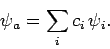(860)

In one dimension, the expansion coefficients take the form (see Sect. 4.9)

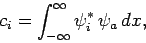$\begin{displaymath} c_i = \int_{-\infty}^\infty\psi_i^\ast \psi_a dx, \end{displaymath}$

(861)

whereas in three dimensions we get

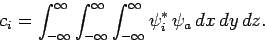$\begin{displaymath} c_i = \int_{-\infty}^\infty\int_{-\infty}^\infty\int_{-\infty}^\infty\psi_i^\ast \psi_a dx dy dz. \end{displaymath}$

(862)

Finally, if $\psi$ is a spinor then we have

$\begin{displaymath} c_i = \psi_i^\dag \psi_a. \end{displaymath}$

(863)

We can represent all of the above possibilities by writing

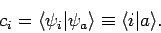$\begin{displaymath} c_i =\langle\psi_i\vert\psi_a\rangle\equiv \langle i\vert a\rangle. \end{displaymath}$

(864)

The expansion (860) thus becomes

$\begin{displaymath} \psi_a = \sum_i\langle\psi_i\vert\psi_a\rangle \psi_i\equiv \sum_i \langle i\vert a\rangle \psi_i. \end{displaymath}$

(865)

Incidentally, it follows that

$\begin{displaymath} \langle i\vert a\rangle^\ast=\langle a\vert i\rangle. \end{displaymath}$

(866)

Finally, if is a general operator, and the wavefunction $\psi_a$ is expanded in the manner shown in Eq. (860), then the expectation value of is written (see Sect. 4.9)

$\begin{displaymath} \langle A\rangle = \sum_{i,j} c_i^\ast c_j A_{ij}. \end{displaymath}$

(867)

Here, the $A_{ij}$ are unsurprisingly known as the matrix elements of

. In one dimension, the matrix elements take the form

$\begin{displaymath} A_{ij} = \int_{-\infty}^\infty\psi_i^\ast A \psi_j dx, \end{displaymath}$

(868)

whereas in three dimensions we get

$\begin{displaymath} A_{ij} = \int_{-\infty}^\infty\int_{-\infty}^\infty\int_{-\infty}^\infty\psi_i^\ast A \psi_j dx dy dz. \end{displaymath}$

(869)

Finally, if $\psi$ is a spinor then we have

$\begin{displaymath} A_{ij}=\psi_i^\dag A \psi_j. \end{displaymath}$

(870)

We can represent all of the above possibilities by writing

$\begin{displaymath} A_{ij}=\langle \psi_i\vert A\vert\psi_j\rangle \equiv \langle i\vert A\vert j\rangle. \end{displaymath}$

(871)

The expansion (867) thus becomes

$\begin{displaymath} \langle A\rangle \equiv\langle a\vert A\vert a\rangle= \sum_... ...rangle \langle i\vert A\vert j\rangle \langle j\vert a\rangle. \end{displaymath}$

(872)

Incidentally, it follows that [see Eq. (194)]

$\begin{displaymath} \langle i\vert A\vert j\rangle^\ast=\langle j\vert A^\dag \vert i\rangle. \end{displaymath}$

(873)

Finally, it is clear from Eq. (872) that

$\begin{displaymath} \sum_{i} \vert i\rangle \langle i\vert \equiv 1, \end{displaymath}$

(874)

where the $\psi_i$ are a complete set of eigenstates, and 1 is the identity operator.

Next: Two-State System Up: Time-Independent Perturbation Theory Previous: Introduction

Richard Fitzpatrick 2010-07-20