


Next: Square Potential Barrier
Up: One-Dimensional Potentials
Previous: Introduction
Infinite Potential Well
Consider a particle of mass  and energy
  moving in the following simple potential:
![\begin{displaymath}
V(x) = \left\{\begin{array}{lcl}
0&\mbox{\hspace{1cm}}&\mbox...
...leq a$}\ [0.5ex]
\infty&&\mbox{otherwise}
\end{array}\right..
\end{displaymath}](img788.png) |
(302) |
It follows from Eq. (301) that if  (and, hence,
  ) is
to remain finite then must go to zero in regions where the potential
is infinite. Hence,
) is
to remain finite then must go to zero in regions where the potential
is infinite. Hence,  in the regions
  and
and  .
Evidently, the problem is equivalent to that of a particle trapped in a
one-dimensional box of length
.
Evidently, the problem is equivalent to that of a particle trapped in a
one-dimensional box of length  .
The boundary conditions on in
the region
.
The boundary conditions on in
the region  are
are
 |
(303) |
Furthermore, it follows from Eq. (301) that satisfies
 |
(304) |
in this region, where
 |
(305) |
Here, we are assuming that  . It is easily demonstrated that there are
no solutions with
. It is easily demonstrated that there are
no solutions with  which are capable of satisfying the boundary conditions (303).
The solution to Eq. (304), subject to the boundary conditions
(303), is
 |
(306) |
where the  are arbitrary (real) constants, and
 |
(307) |
for
 . Now, it can be seen from Eqs. (305) and (307)
that the energy is only allowed to take certain discrete values:
i.e.,
. Now, it can be seen from Eqs. (305) and (307)
that the energy is only allowed to take certain discrete values:
i.e.,
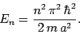 |
(308) |
In other words, the eigenvalues of the energy operator are discrete. This
is a general feature of bounded solutions: i.e., solutions in which
 as
as
 . According to the discussion in Sect. 4.12,
we expect the stationary eigenfunctions
. According to the discussion in Sect. 4.12,
we expect the stationary eigenfunctions  to satisfy
the orthonormality constraint
to satisfy
the orthonormality constraint
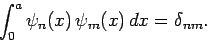 |
(309) |
It is easily demonstrated that this is the case, provided
 .
Hence,
.
Hence,
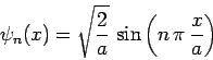 |
(310) |
for
.
Finally, again from Sect. 4.12, the general time-dependent solution can be written as a linear superposition of stationary solutions:
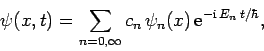 |
(311) |
where
 |
(312) |
Next: Square Potential Barrier
Up: One-Dimensional Potentials
Previous: Introduction
Richard Fitzpatrick
2010-07-20