


Next: Electric Dipole Approximation
Up: Time-Dependent Perturbation Theory
Previous: Harmonic Perturbations
Let us use some of the results of time-dependent perturbation theory
to investigate the interaction of an atomic electron with
classical (i.e., non-quantized) electromagnetic radiation.
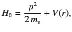
The unperturbed Hamiltonian
is
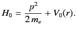 |
(862) |
The standard classical prescription for obtaining the Hamiltonian of
a particle
of charge  in the presence of an electromagnetic field is
where
 is the vector potential and
 is the scalar potential. Note that
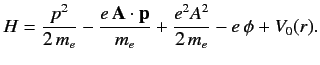
This prescription also works in quantum mechanics. Thus, the Hamiltonian
of an atomic electron placed in an electromagnetic field is
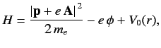 |
(867) |
where  and
and  are real functions of the position operators.
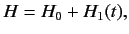
The above equation can be written
are real functions of the position operators.
The above equation can be written
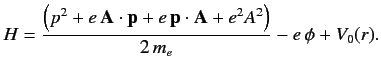 |
(868) |
Now,
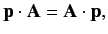 |
(869) |
provided that we adopt the gauge
 .
Hence,
.
Hence,
 |
(870) |
Suppose that the perturbation corresponds to a monochromatic plane-wave, for which
where
 and
and  are unit vectors that specify the direction
of polarization and the direction of propagation, respectively.
Note that
are unit vectors that specify the direction
of polarization and the direction of propagation, respectively.
Note that
 . The Hamiltonian
becomes
. The Hamiltonian
becomes
 |
(873) |
with
 |
(874) |
and
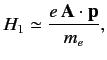 |
(875) |
where the  term, which is second order in
  , has been neglected.
The perturbing Hamiltonian can be written
![$\displaystyle H_1 = \frac{e \,A_0\, \mbox{\boldmath$\epsilon$}\cdot{\bf p} }{m_...
...\exp[-{\rm i}\,(\omega/c)\, {\bf n}\cdot{\bf x} + {\rm i}\, \omega\, t]\right).$](img2050.png) |
(876) |
This has the same form as Equation (850), provided that
![$\displaystyle V = - \frac{e \,A_0\, \mbox{\boldmath$\epsilon$}\cdot{\bf p} }{m_e}\, \exp[-{\rm i}\,(\omega/c)\, {\bf n}\cdot{\bf x}\,]$](img2051.png) |
(877) |
It is clear, by analogy with the previous analysis, that the first
term on the right-hand side of Equation (876) describes the absorption
of a photon of energy
 , whereas the second term describes
the stimulated emission of a photon of energy
. It follows from
Equations (859) and (860) that the rates of absorption and stimulated emission are
, whereas the second term describes
the stimulated emission of a photon of energy
. It follows from
Equations (859) and (860) that the rates of absorption and stimulated emission are
and
respectively.
Now, the energy density of a radiation field
is
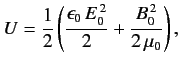 |
(880) |
where  and
and
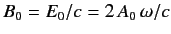 are the peak electric and magnetic field-strengths,
respectively. Hence,
are the peak electric and magnetic field-strengths,
respectively. Hence,
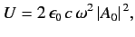 |
(881) |
and expressions (878) and (879)
become
and
respectively.
Finally, if we imagine that the incident radiation has a range of different frequencies, so
that
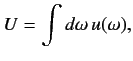 |
(884) |
where
 is the energy density of radiation whose frequency lies in the range
  to
to
 , then we can integrate our transition rates over
to give
, then we can integrate our transition rates over
to give
for absorption, and
for stimulated emission. Here,
 and
and
 .
Furthermore, we are assuming that the radiation is incoherent, so that intensities can be
added.
.
Furthermore, we are assuming that the radiation is incoherent, so that intensities can be
added.
Next: Electric Dipole Approximation
Up: Time-Dependent Perturbation Theory
Previous: Harmonic Perturbations
Richard Fitzpatrick
2013-04-08
![$\displaystyle w_{i\rightarrow n} = \frac{\pi}{\hbar^2} \frac{e^2}{\epsilon_0\,m...
..., \vert\langle n\vert\, \exp[\,{\rm i}\,(\omega_{ni}/c)\,{\bf n}\cdot{\bf x}]\,$](img2065.png)
![$\displaystyle w_{i\rightarrow n} = \frac{\pi}{\hbar^2} \frac{e^2}{\epsilon_0\,m...
...\, \vert\langle n\vert\, \exp[-{\rm i}\,(\omega_{in}/c)\,{\bf n}\cdot{\bf x}]\,$](img2067.png)
![$\displaystyle w_{i\rightarrow n} = \frac{2\pi}{\hbar} \frac{e^2}{m_e^{\,2}}\, \...
...\,2}\, \vert\langle n\vert\, \exp[\,{\rm i}\,(\omega/c)\,{\bf n}\cdot{\bf x}]\,$](img2052.png)
![$\displaystyle w_{i\rightarrow n} = \frac{2\pi}{\hbar} \frac{e^2}{m_e^{\,2}}\, \...
...{\,2}\, \vert\langle n\vert\, \exp[-{\rm i}\,(\omega/c)\,{\bf n}\cdot{\bf x}]\,$](img2054.png)
![$\displaystyle w_{i\rightarrow n} = \frac{\pi}{\hbar} \frac{e^2}{\epsilon_0\,m_e...
...\, U\, \vert\langle n\vert\, \exp[\,{\rm i}\,(\omega/c)\,{\bf n}\cdot{\bf x}]\,$](img2060.png)
![$\displaystyle w_{i\rightarrow n} = \frac{\pi}{\hbar} \frac{e^2}{\epsilon_0\,m_e...
...}\, U\, \vert\langle n\vert\, \exp[-{\rm i}\,(\omega/c)\,{\bf n}\cdot{\bf x}]\,$](img2061.png)