Consider a system in a state ![]() that evolves in time. At time
that evolves in time. At time
![]() , the state of the system is represented by the ket
, the state of the system is represented by the ket
![]() . The label
. The label
![]() is needed to distinguish this ket from any other ket (
is needed to distinguish this ket from any other ket (
![]() , say)
that is evolving in time. The label
, say)
that is evolving in time. The label ![]() is needed to distinguish the different
states of the system at different times.
is needed to distinguish the different
states of the system at different times.
The final state of the system at time ![]() is completely determined by its
initial state at time
is completely determined by its
initial state at time ![]() plus the time interval
plus the time interval ![]() (assuming that
the system is left undisturbed during this time interval). However, the
final state only determines the direction of the final state ket.
Even if we adopt the convention that all state kets have unit norms,
the final ket is still not completely determined, because it can be multiplied
by an arbitrary
phase-factor. However, we expect that if a superposition relation
holds for certain states at time
(assuming that
the system is left undisturbed during this time interval). However, the
final state only determines the direction of the final state ket.
Even if we adopt the convention that all state kets have unit norms,
the final ket is still not completely determined, because it can be multiplied
by an arbitrary
phase-factor. However, we expect that if a superposition relation
holds for certain states at time ![]() then the same relation
should hold between the corresponding time-evolved states at time
then the same relation
should hold between the corresponding time-evolved states at time ![]() , assuming
that the system is left undisturbed between times
, assuming
that the system is left undisturbed between times ![]() and
and ![]() .
In other words,
if
.
In other words,
if
According to Equations (220) and (221), the final ket
![]() depends linearly
on the initial ket
depends linearly
on the initial ket
![]() . Thus, the final ket can be regarded as the
result of some linear operator acting on the initial ket: i.e.,
. Thus, the final ket can be regarded as the
result of some linear operator acting on the initial ket: i.e.,
Because we have adopted a convention in which the norm of any state ket is unity,
it make sense to define the time evolution operator ![]() in such a manner that
it preserves the length of any ket upon which it acts
(i.e., if a ket is properly normalized at time
in such a manner that
it preserves the length of any ket upon which it acts
(i.e., if a ket is properly normalized at time ![]() then it will remain normalized at
all subsequent times
then it will remain normalized at
all subsequent times ![]() ).
This is always possible,
because the length of a ket possesses no physical significance. Thus,
we require that
).
This is always possible,
because the length of a ket possesses no physical significance. Thus,
we require that
| (223) |
Up to now, the time evolution operator ![]() looks very much like the
spatial displacement
operator
looks very much like the
spatial displacement
operator ![]() introduced in the previous section. However, there are some
important differences between time evolution and spatial displacement. In general,
we do expect the expectation value of some observable
introduced in the previous section. However, there are some
important differences between time evolution and spatial displacement. In general,
we do expect the expectation value of some observable ![]() to
evolve with time, even if the system is left in a state of undisturbed motion
(after all, time evolution has no meaning unless something observable
changes with time). The triple product
to
evolve with time, even if the system is left in a state of undisturbed motion
(after all, time evolution has no meaning unless something observable
changes with time). The triple product
![]() can evolve
either because the ket
can evolve
either because the ket ![]() evolves and the operator
evolves and the operator ![]() stays constant,
the ket
stays constant,
the ket ![]() stays constant and the operator
stays constant and the operator ![]() evolves, or both
the ket
evolves, or both
the ket ![]() and the operator
and the operator ![]() evolve.
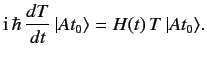
Because we are already committed to evolving state kets, according to Equation (222),
let us assume that the time evolution operator
evolve.
Because we are already committed to evolving state kets, according to Equation (222),
let us assume that the time evolution operator ![]() can be chosen in such a
manner that the operators representing the dynamical variables of the
system do not
evolve in time (unless they contain some specific time dependence).
can be chosen in such a
manner that the operators representing the dynamical variables of the
system do not
evolve in time (unless they contain some specific time dependence).
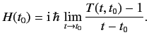
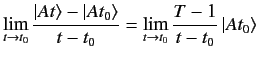
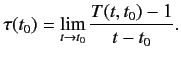
We expect, from physical continuity, that if
![]() then
then
![]() for any ket
for any ket ![]() . Thus, the
limit
. Thus, the
limit
| (227) |
 |
(228) |
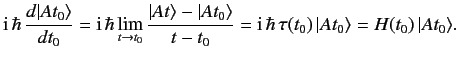
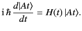
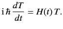
Equation (229) gives the general law for the time evolution of a state
ket in a scheme in which the operators representing the dynamical variables remain
fixed. This equation is denoted the Schrödinger equation of motion.
It involves a Hermitian operator ![]() which is, presumably, a characteristic
of the dynamical system under investigation.
which is, presumably, a characteristic
of the dynamical system under investigation.
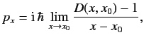
We saw, in Section 2.8, that
if the operator ![]() displaces the system along the
displaces the system along the ![]() -axis from
-axis from ![]() to
to ![]() then
then
 |
(230) |
 |
(231) |
Substituting
![]() into Equation (229) yields
into Equation (229) yields
 |
(232) |
![$\displaystyle T(t, t_0) = \exp\left[-\frac{{\rm i}}{\hbar} \int_{t_0}^t dt'\,H(t') \right],$](img561.png)