Next: Optical Theorem
Up: Scattering Theory
Previous: Born Expansion
Partial Waves
We can assume, without loss of generality, that the incident wavefunction
is characterized by a wavevector,  , that is aligned parallel to the
  -axis.
The scattered wavefunction is characterized by a wavevector,
-axis.
The scattered wavefunction is characterized by a wavevector,  ,
that has the same magnitude as
, but, in general, points
in a different direction. The direction of
is specified
by the polar angle
,
that has the same magnitude as
, but, in general, points
in a different direction. The direction of
is specified
by the polar angle  (i.e., the angle subtended between the
two wavevectors), and an azimuthal angle
(i.e., the angle subtended between the
two wavevectors), and an azimuthal angle  measured about the
-axis.
Equations (10.33) and (10.34) strongly suggest that for a spherically symmetric
scattering potential [i.e.,
measured about the
-axis.
Equations (10.33) and (10.34) strongly suggest that for a spherically symmetric
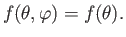
scattering potential [i.e.,
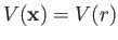 ], the scattering amplitude
is a function of
only: that is,
], the scattering amplitude
is a function of
only: that is,
 |
(10.53) |
Let us assume that this is the case.
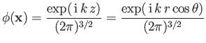
It follows that neither the incident wavefunction,
 |
(10.54) |
[see Equation (10.14)], nor the total wavefunction far from the scattering region,
![$\displaystyle \psi({\bf x}) = \frac{1}{(2\pi)^{3/2}} \left[ \exp(\,{\rm i}\,k\,r\cos\theta) + \frac{\exp(\,{\rm i}\,k\,r)\, f(\theta)} {r} \right]$](img3518.png) |
(10.55) |
[see Equation (10.20)], depend on the azimuthal angle,
.
Outside the range of the scattering potential,
 and
and
 both satisfy the free-space Schrödinger equation,
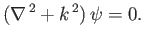 |
(10.56) |
Consider the most general solution to this equation that is independent of the azimuthal angle,
.
Separation of variables (in spherical coordinates) yields
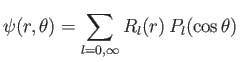 |
(10.57) |
(See Exercise 10.)
The Legendre polynomials,
 , are related to the
associated Legendre functions,
, are related to the
associated Legendre functions,
 , as well as the spherical harmonics,
 , introduced in Section 4.4, via
 , and
, and
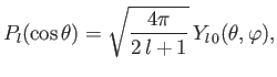 |
(10.58) |
respectively.
Equations (10.56) and (10.57) can be combined to give
![$\displaystyle r^{\,2} \,\frac{d^{\,2} R_l}{dr^{\,2}} + 2\,r\,\frac{dR_l}{dr} + [k^{\,2} \,r^{\,2} - l\,(l+1)]\,R_l = 0.$](img3525.png) |
(10.59) |
(See Exercise 10.)
The two independent solutions to this equation are the
spherical Bessel function,  , and the Neumann function,
 ,
where
,
where
[1].
Note that spherical Bessel functions are well behaved in the limit
 , whereas Neumann functions become singular.
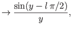
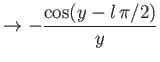
The asymptotic behavior of these functions in the limit
, whereas Neumann functions become singular.
The asymptotic behavior of these functions in the limit
 is
is
[1].
We can write
 |
(10.64) |
where the  are constants. Of course, there are no Neumann functions in
this expansion because they are not well behaved as
are constants. Of course, there are no Neumann functions in
this expansion because they are not well behaved as
 (whereas the function on the
left-hand side is clearly finite at
(whereas the function on the
left-hand side is clearly finite at  ).
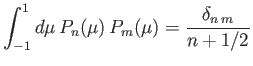
As is well known, the Legendre polynomials are orthogonal functions,
).
As is well known, the Legendre polynomials are orthogonal functions,
 |
(10.65) |
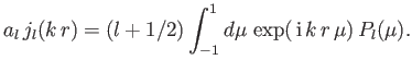
[1], so we can invert the preceding expansion to give
 |
(10.66) |
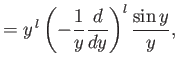
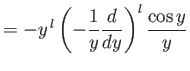
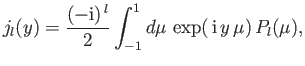
Now,
 |
(10.67) |
for
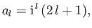
 [1]. Thus, a comparison of the previous two equations yields
 |
(10.68) |
giving
 |
(10.69) |
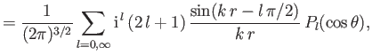
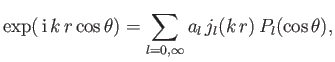
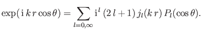
The preceding expression specifies how
a plane wave can be decomposed into
a series of spherical waves. The latter waves are usually referred to as partial waves.
The most general expression for the total wavefunction outside the
scattering region is
![$\displaystyle \psi({\bf x}) = \frac{1}{(2\pi)^{3/2}} \sum_{l=0,\infty}\left[ A_l\,j_l(k\,r) + B_l\,\eta_l(k\,r)\right] P_l(\cos\theta),$](img3542.png) |
(10.70) |
where the  and
and  are constants.
Note that the Neumann functions are allowed to appear
in this expansion, because
its region of validity does not include the origin. In the large-
are constants.
Note that the Neumann functions are allowed to appear
in this expansion, because
its region of validity does not include the origin. In the large- limit, the total wavefunction reduces to
![$\displaystyle \psi ({\bf x} ) \simeq \frac{1}{(2\pi)^{3/2}} \sum_{l=0,\infty}\l...
...\pi/2)}{k\,r} - B_l\,\frac{\cos(k\,r -l\,\pi/2)}{k\,r} \right] P_l(\cos\theta),$](img3545.png) |
(10.71) |
where use has been made of Equations (10.62) and (10.63). The previous expression can also
be written
 |
(10.72) |
where
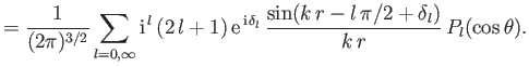
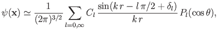
Equation (10.72) yields
![$\displaystyle \psi({\bf x}) \simeq \frac{1}{(2\pi)^{3/2}} \sum_{l=0,\infty} C_l...
...rm i}\,(k\,r - l\,\pi/2+ \delta_l)} }{2\,{\rm i}\,k\,r}\right] P_l(\cos\theta),$](img3551.png) |
(10.75) |
which contains both incoming and outgoing spherical waves. What is the
source of the incoming waves? Obviously, they must form part of
the large-
asymptotic expansion of the incident wavefunction. In fact,
it is easily seen from Equations (10.54), (10.62), and (10.69) that
![$\displaystyle \phi({\bf x}) \simeq \frac{1}{(2\pi)^{3/2}} \sum_{l=0,\infty} {\r...
...{\rm e}^{-{\rm i}\,(k\,r - l\,\pi/2)}}{2\,{\rm i}\,k\,r}\right]P_l(\cos\theta),$](img3552.png) |
(10.76) |
in the large-
limit. Now, Equations (10.54) and (10.55) give
![$\displaystyle (2\pi)^{3/2}\,[\psi({\bf x} )- \phi({\bf x}) ] = \frac{\exp(\,{\rm i}\,k\,r)}{r}\, f(\theta).$](img3553.png) |
(10.77) |
Note that the right-hand side consists only of an outgoing spherical
wave. This implies that the coefficients of the incoming spherical waves
in the large-
expansions of
and
must be equal. It follows from Equations (10.75) and (10.76) that
![$\displaystyle C_l = (2\,l+1)\,\exp[\,{\rm i}\,(\delta_l + l\,\pi/2)],$](img3554.png) |
(10.78) |
which leads to
Thus, it is apparent that the effect of the scattering is to introduce a phase-shift,  , into the
 th partial wave.
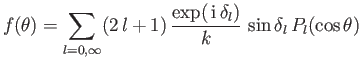
Finally, Equation (10.77) yields
th partial wave.
Finally, Equation (10.77) yields
 |
(10.81) |
[42].
Clearly, determining the scattering amplitude,
 , via a decomposition into
partial waves (i.e., spherical waves), is equivalent to determining
the phase-shifts,
.
, via a decomposition into
partial waves (i.e., spherical waves), is equivalent to determining
the phase-shifts,
.
It is helpful to write
where
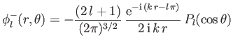 |
(10.84) |
is an ingoing spherical wave, whereas
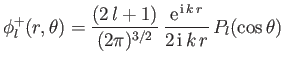 |
(10.85) |
is an outgoing spherical wave. Moreover,
 |
(10.86) |
[See Equations (10.79) and (10.80).]
Note that
 and
and
 are both eigenstates of the magnitude of the total
orbital angular momentum about the origin belonging to the eigenvalues
are both eigenstates of the magnitude of the total
orbital angular momentum about the origin belonging to the eigenvalues
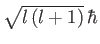 . (See Chapter 4.)
Thus, in preforming a partial wave expansion, we have effectively separated the incoming and outgoing particles into
streams possessing definite angular momenta about the origin. Moreover, the effect of the scattering is to introduce an
angular-momentum-dependent
phase-shift into the outgoing particle streams.
. (See Chapter 4.)
Thus, in preforming a partial wave expansion, we have effectively separated the incoming and outgoing particles into
streams possessing definite angular momenta about the origin. Moreover, the effect of the scattering is to introduce an
angular-momentum-dependent
phase-shift into the outgoing particle streams.
The net outward particle flux through a sphere of radius
, centered on the origin, is proportional to
 |
(10.87) |
where
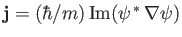 is the probability current. It follows that
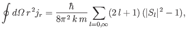 |
(10.88) |
where use has been made of Equation (10.65).
Of course, the net particle flux must be zero, otherwise the number of particles would not be
conserved. Particle conservation is ensured by the fact that  for all
. [See Equation (10.86).]
for all
. [See Equation (10.86).]
Next: Optical Theorem
Up: Scattering Theory
Previous: Born Expansion
Richard Fitzpatrick
2016-01-22
![$\displaystyle =\sum_{l=0,\infty} \left[\phi_l^+(r,\theta)+\phi_l^-(r,\theta)\right],$](img3562.png)
![$\displaystyle =\sum_{l=0,\infty} \left[S_l\,\phi_l^+(r,\theta)+\phi_l^-(r,\theta)\right],$](img3564.png)