Next: Closure in Collisionless Magnetized Up: Plasma Fluid Theory Previous: MHD Equations Contents
If we assume that
 then the dominant term in the electron energy conservation equation
(4.202) yields
then the dominant term in the electron energy conservation equation
(4.202) yields
 |
(4.206) |
The dominant term in the ion energy conservation equation (4.205) yields
 |
(4.208) |
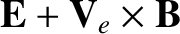
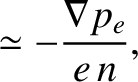
The dominant terms in the electron and ion momentum conservation equations, (4.201) and (4.204), yield
The sum of the preceding two equations gives
 |
(4.212) |
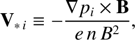
 . In other words, in the drift approximation, to lowest order, the plasma exists in an equilibrium state in which
the magnetic force density balances the total scalar pressure force density. It follows from the previous equation that
. In other words, in the drift approximation, to lowest order, the plasma exists in an equilibrium state in which
the magnetic force density balances the total scalar pressure force density. It follows from the previous equation that
 |
(4.213) |
 , and making use of Equations (4.207) and (4.209), we deduce that
 |
(4.214) |
 and
and
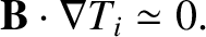
 , are also constant along magnetic
field-lines. Hence, Equation (4.210) yields
, are also constant along magnetic
field-lines. Hence, Equation (4.210) yields
 |
(4.215) |
Equations (4.210)–(4.211) can be inverted to give
Here,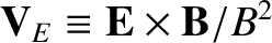 is the
 velocity, whereas
 |
(4.218) |
 |
(4.219) |
According to Equations (4.216)–(4.217), in the drift approximation, the velocity of the electron
fluid perpendicular to the magnetic field is the sum of the
velocity and the electron diamagnetic velocity. A similar statement can be made for the ion fluid.
By contrast, in the MHD approximation the perpendicular velocities of the
two fluids consist of the
velocity alone, and are,
therefore, identical to lowest order. The main difference between the
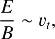
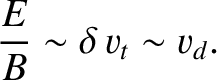
two orderings lies in the assumed magnitude of the electric field. In the
MHD limit
 |
(4.220) |
 |
(4.221) |
The diamagnetic velocities are so named because the diamagnetic current,
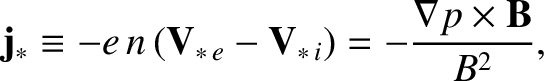 |
(4.222) |
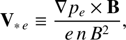
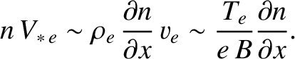
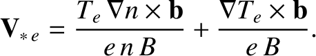
The electron diamagnetic velocity can be written
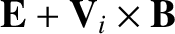
In order to account for this velocity, let us consider a simplified case in which the electron temperature is uniform, there is a uniform density gradient running along the -direction, and the magnetic
field is parallel to the
-direction, and the magnetic
field is parallel to the  -axis. (See Figure 4.3.)
The electrons gyrate in the -
-axis. (See Figure 4.3.)
The electrons gyrate in the - plane in circles of radius
 . At a given point, coordinate
  , say, on the -axis,
the electrons that come from the right and the left have traversed distances
of approximate magnitude
, say, on the -axis,
the electrons that come from the right and the left have traversed distances
of approximate magnitude  . Thus, the electrons from the right originate from
regions where the particle density is approximately
. Thus, the electrons from the right originate from
regions where the particle density is approximately
 greater than the regions from which the electrons from the left originate.
It follows that the -directed particle flux
is unbalanced, with slightly more particles moving in the
greater than the regions from which the electrons from the left originate.
It follows that the -directed particle flux
is unbalanced, with slightly more particles moving in the  -direction
than in the
-direction
than in the  -direction. Thus, there is a net particle flux
in the -direction: that is, in the direction of
-direction. Thus, there is a net particle flux
in the -direction: that is, in the direction of
 .
The magnitude of this flux is
.
The magnitude of this flux is
 |
(4.224) |
-direction, because the
-directed fluxes are associated with electrons that originate from regions
where  . We have now accounted for the first term on the
right-hand side of Equation (4.223).
We can account for the second term using similar arguments.
The ion diamagnetic velocity is similar in magnitude to the electron
diamagnetic velocity, but is oppositely directed, because ions gyrate
in the opposite direction to electrons.
. We have now accounted for the first term on the
right-hand side of Equation (4.223).
We can account for the second term using similar arguments.
The ion diamagnetic velocity is similar in magnitude to the electron
diamagnetic velocity, but is oppositely directed, because ions gyrate
in the opposite direction to electrons.
The most curious aspect of diamagnetic flows is that they represent fluid flows for which there is no corresponding motion of the particle guiding centers. Nevertheless, the diamagnetic velocities are real fluid velocities, and the associated diamagnetic current is a real current. For instance, the diamagnetic current contributes to force balance inside the plasma, and also gives rise to ohmic heating.

![$\displaystyle m_e\, n\,\frac{\partial {\bf V}_e}{\partial t} +
m_e\, n\,({\bf V}_e\cdot\nabla){\bf V}_e+
[\delta^{-2}]\,\nabla p_e+
[\zeta^{-1}]\, \nabla\cdot$](img1498.png)


![$\displaystyle + [\delta^{-2}]\,e \,n\,
({\bf E} + {\bf V}_e\times {\bf B})$](img1458.png)
![$\displaystyle =[\delta^{-2}\,\zeta]\, {\bf F}_U + [\delta^{-2}]\,
{\bf F}_T,$](img1459.png)
![$\displaystyle + [\zeta^{-1}]\,\nabla\cdot{\bf q}_{Te} +\nabla\cdot{\bf q}_{Ue}$](img1499.png)
![$\displaystyle =-[\delta^{-2}\,\zeta\,\mu^2]\, w_i
+[\zeta]\,w_U + w_T,$](img1461.png)
![$\displaystyle m_i \,n\,\frac{\partial {\bf V}_i}{\partial t} +
m_i \,n\,({\bf V}_i\cdot\nabla) {\bf V}_i +
[\delta^{-2}]\,\nabla p_i +
[\zeta^{-1}]\,\nabla\cdot$](img1500.png)

![$\displaystyle - [\delta^{-2}]\,e\, n\,
({\bf E} + {\bf V}_i\times {\bf B})$](img1464.png)
![$\displaystyle = -[\delta^{-2}\,\zeta]\, {\bf F}_U - [\delta^{-2}]\,{\bf F}_T,$](img1465.png)
![$\displaystyle \frac{3}{2}\frac{\partial p_i}{\partial t} + \frac{3}{2}
\,({\bf ...
...i
+ \frac{5}{2}\,p_i\,\nabla\cdot{\bf V}_i
+ [\zeta^{-1}]\,\nabla\cdot{\bf q}_i$](img1501.png)
![$\displaystyle = [\delta^{-2}\,\zeta\,\mu^2]\,w_i.$](img1502.png)


![\includegraphics[height=3in]{Chapter04/fig4_3.eps}](img1533.png)