Next: Cold-Plasma Dielectric Permittivity Up: Waves in Cold Plasmas Previous: Introduction Contents
Consider a homogeneous, magnetized, quasi-neutral plasma, consisting of equal
numbers of electrons and ions, in which the mean velocities of both plasma species are zero.
It follows that
 , and
, and
 , where the subscript 0 denotes an equilibrium quantity.
In a homogeneous medium, the
general solution of a system of linear equations can be constructed as
a superposition of plane wave solutions of the form (Fitzpatrick 2013)
, where the subscript 0 denotes an equilibrium quantity.
In a homogeneous medium, the
general solution of a system of linear equations can be constructed as
a superposition of plane wave solutions of the form (Fitzpatrick 2013)
 and
and
 .
Here,
.
Here,  ,
,  , and
, and  are the perturbed electric field, magnetic field, and
plasma center-of-mass velocity, respectively.
The
surfaces of constant phase,
are the perturbed electric field, magnetic field, and
plasma center-of-mass velocity, respectively.
The
surfaces of constant phase,
 |
(5.2) |
 , traveling at the velocity
 |
(5.3) |
 , and
, and
 is a unit vector
pointing in the direction of . Here,
is a unit vector
pointing in the direction of . Here,
 is termed the phase-velocity of the wave (Fitzpatrick 2013).
Henceforth, for ease of notation, we shall omit
the subscript from field variables.
is termed the phase-velocity of the wave (Fitzpatrick 2013).
Henceforth, for ease of notation, we shall omit
the subscript from field variables.
Substitution of the plane-wave solution (5.1) into Maxwell's equations yields
where is the perturbed current density.
In linear theory, the current is related to the electric field via
where the electrical conductivity tensor,
is the perturbed current density.
In linear theory, the current is related to the electric field via
where the electrical conductivity tensor,
 , is a
function of both and
, is a
function of both and  . In the presence of a non-zero equilibrium
magnetic field, this tensor is anisotropic in nature.
. In the presence of a non-zero equilibrium
magnetic field, this tensor is anisotropic in nature.
Substitution of Equation (5.6) into Equation (5.4) yields
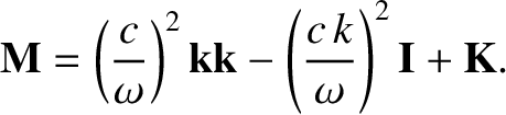
where is termed the dielectric permittivity tensor. Here, is the identity tensor. Eliminating the
magnetic field between Equations (5.5) and (5.7), we obtain
where
is the identity tensor. Eliminating the
magnetic field between Equations (5.5) and (5.7), we obtain
where
The solubility condition for Equation (5.9),
 |
(5.11) |
, to the wavevector, .
Also, as the name
“dispersion relation” suggests, this relation allows us to determine the rate at which the
different Fourier components of a wave pulse disperse due to
the variation of their phase-velocity with frequency (Fitzpatrick 2013).
![$\displaystyle {\bf E} ({\bf r}, t) = {\bf E}_{\bf k} \,\exp[\,{\rm i}\,({\bf k}
\cdot{\bf r} - \omega\, t)],$](img1662.png)