Next: Ionospheric Radio Wave Propagation
Up: Wave Propagation Through Inhomogeneous
Previous: Pulse Propagation
Ray Tracing
Let us now generalize the preceding analysis so that we can deal with pulse
propagation though a three-dimensional magnetized plasma.
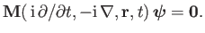
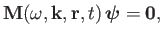
A general wave problem can be written as a set of  coupled, linear, homogeneous,
first-order, partial-differential equations, which take the form (Hazeltine and Waelbroeck 2004)
coupled, linear, homogeneous,
first-order, partial-differential equations, which take the form (Hazeltine and Waelbroeck 2004)
 |
(6.87) |
The vector-field
 has
components (e.g.,
has
components (e.g.,
 might consist of
  ,
,  ,
,  , and
, and  ) characterizing
some small disturbance, and
) characterizing
some small disturbance, and  is an
is an  matrix characterizing the
undisturbed plasma.
matrix characterizing the
undisturbed plasma.
The lowest order WKB approximation is premised on the assumption that
depends so weakly on  and
and  that all of the
spatial and temporal dependence of the components of
that all of the
spatial and temporal dependence of the components of
 is specified by a common factor
 .
Thus,
Equation (6.87) reduces to
.
Thus,
Equation (6.87) reduces to
 |
(6.88) |
where
In general, Equation (6.88) has many solutions, corresponding to the many different
types and polarizations of waves that can propagate through the plasma in question,
all of which satisfy the dispersion relation
 |
(6.91) |
where
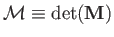 .
As is easily demonstrated (see Section 6.2), the WKB approximation is valid
provided that the characteristic
variation lengthscale and variation timescale of the plasma are much longer than
the wavelength,
.
As is easily demonstrated (see Section 6.2), the WKB approximation is valid
provided that the characteristic
variation lengthscale and variation timescale of the plasma are much longer than
the wavelength,  , and the period,
 , respectively,
of the wave in question.
, respectively,
of the wave in question.
Let us concentrate on one particular solution of Equation (6.88) (e.g.,
on one particular type of plasma wave). For this solution, the dispersion
relation (6.91) yields
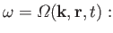 |
(6.92) |
that is, the dispersion relation yields a
unique frequency for a wave of a given wave-vector,  , located
at a given point,
, located
at a given point,
 , in space and time. There is also a unique
associated
with this frequency, which is obtained from Equation (6.88). To lowest order, we can
neglect the variation of
with
and
.
A general pulse solution is written
, in space and time. There is also a unique
associated
with this frequency, which is obtained from Equation (6.88). To lowest order, we can
neglect the variation of
with
and
.
A general pulse solution is written
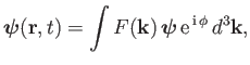 |
(6.93) |
where (locally)
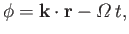 |
(6.94) |
and
 is a function that specifies the initial structure of the pulse
in
-space.
is a function that specifies the initial structure of the pulse
in
-space.
The integral (6.93) averages to zero, except at a point of stationary
phase, where
 . (See Section 6.7.) Here,
 is the
-space
gradient operator. It follows that the (instantaneous) trajectory of the pulse
matches that of a point of stationary phase:
is the
-space
gradient operator. It follows that the (instantaneous) trajectory of the pulse
matches that of a point of stationary phase:
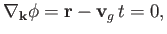 |
(6.95) |
where
 |
(6.96) |
is the group-velocity. Thus, the instantaneous velocity of a pulse is
always
equal to the local group-velocity.
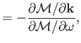
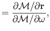
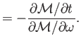
Let us now determine how the wavevector,
, and the angular frequency,  ,
of a pulse evolve as the pulse propagates through the
plasma. We start from the cross-differentiation rules
[see Equations (6.89) and (6.90)]:
,
of a pulse evolve as the pulse propagates through the
plasma. We start from the cross-differentiation rules
[see Equations (6.89) and (6.90)]:
Equations (6.92), (6.97), and (6.98) yield [making use of the Einstein summation
convention (Riley 1974)]
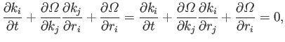 |
(6.99) |
or
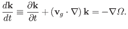 |
(6.100) |
In other words, the variation of
, as seen in a frame co-moving with
the pulse, is determined by the spatial gradients in
 .
.
Partial differentiation of Equation (6.92) with respect to
gives
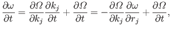 |
(6.101) |
which can be written
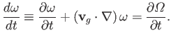 |
(6.102) |
In other words, the variation of
, as seen in a frame co-moving with
the pulse, is determined by the time variation of
.
According to the previous analysis, the evolution of a pulse
propagating though a spatially and temporally non-uniform
plasma can be determined by solving the
ray equations:
The previous equations are conveniently rewritten in terms of the dispersion
relation (6.91) (Hazeltine and Waelbroeck 2004):
Incidentally, the variation in the amplitude of the pulse, as it
propagates through the plasma, can only be determined by expanding
the WKB solutions to higher order. (See Exercises 3 and 4.)
Next: Ionospheric Radio Wave Propagation
Up: Wave Propagation Through Inhomogeneous
Previous: Pulse Propagation
Richard Fitzpatrick
2016-01-23